Data Simulation

10 minute read

Published: January 03, 2025

Bayesian Workflow

This R markdown document gives an idea of how data simulation fits into the Bayesian workflow and how to perform this in R.

Table of content

Overview.

Data stimulation is not inherently Bayesian, but adopted by many Bayesian statisticians to ensure that the models used are sensible. In this R-markdown I demonstrate how data-simulation can be used for a simple linear regression and later for more complex models such as psychometric functions. It is important to stress the importance of simulations, as proper use of simulations can help answer many of the questions people have about their statistical or computational models. These questions could be what sample size would i need to detect an effect size of x, or what what happens to my model if i have a certain type of distributed data etc.

Simulation (Linear model).

In order to start appreciating simulations we start by simulating data from the linear model:

$y_i \sim \mathcal{N}(a + b \cdot x_i , \sigma)$

Here $y_i$ is our outcome of interest and $x_i$ is our independent variable. All other symbols a,b and $\sigma$ are parameters that we in the end want to estimate.

To simulate data from this model we choose values for our parameters and select a range of x-values that would make sense for the experimental design (levels of the independent variable you have in the experiment).

#data points
N = 100
#intercept
a = 10
#slope
b = 3
#sigma
sigma = 20
#x's
x = seq(0,100, length.out = N)

Now to simulate data we use the distributions build into R. In the above we specified that the normal distribution, so we use the random number generator of the normal distribution to get responses $y_i$ .

# generate y-values from our model and parameters
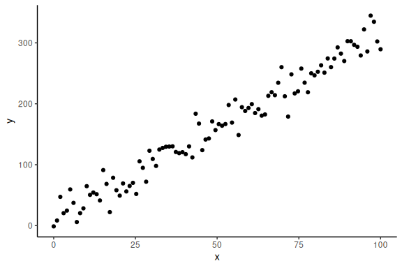
y = rnorm(N,a+b*x,sigma)

Now importantly we can plot it, ensuring ourselves that it makes sense

data.frame() %>% 
  ggplot(aes(x =x,y = y))+
  geom_point()+
  theme_classic()

Now that we have some simulated data, where we know the parameters i.e. a b and $\sigma$ , we can try and fit the model. We start by doing this in the frequentist sense:

# Calling the linear model and plotting as a table
m1 = lm(y~x)
# Making a nice table of the model results
summary(m1)

## 
## Call:
## lm(formula = y ~ x)
## 
## Residuals:
##     Min      1Q  Median      3Q     Max 
## -49.071 -11.047  -0.692  12.970  41.897 
## 
## Coefficients:
##             Estimate Std. Error t value Pr(>|t|)    
## (Intercept)  9.32214    3.63087   2.567   0.0118 *  
## x            3.04972    0.06273  48.616   <2e-16 ***
## ---
## Signif. codes:  0 '***' 0.001 '**' 0.01 '*' 0.05 '.' 0.1 ' ' 1
## 
## Residual standard error: 18.29 on 98 degrees of freedom
## Multiple R-squared:  0.9602, Adjusted R-squared:  0.9598 
## F-statistic:  2364 on 1 and 98 DF,  p-value: < 2.2e-16

Here we get the parameters; a (intercept) and b (the slope). These two estimates are not terribly off the values we put in which where 10 and 3 respectively. To get the last parameter $\sigma$ we can do:

# getting the sigma estimate
sigma(m1)

## [1] 18.2907

Which is also decently close to the 20 which we simulated.

This markdown is not about fitting models to simulated data, but to leverage simulations and explore the meaning of these. In the next section we generalize the scripts for the linear model so we can investigate the meaning of our parameters. This is meant as an exercise to understand one of the ways one can use simulations, i.e. to understand the meaning of the parameters of a model.

Generalized simulations (linear model).

We start with the same linear model as before, but now simulate several parameter pairs (i.e. pairs of a,b and $\sigma$ ).

# keep the number of data points constant (could also vary this)
N = 100
#intercept
a = seq(0,300,length.out = 5)
#slope
b = seq(0,3,length.out = 5)
#sigma
sigma = seq(1,30,length.out = 5)

parameters = expand.grid(a = a,
                         b = b,
                         sigma = sigma,
                         N = N)

#lastly we put it together in a dataframe:
df = parameters %>% rowwise() %>% 
  mutate(x = list(seq(0,100, length.out = N))) %>% unnest(x)

Now the last part is getting the responses i.e. $y_i$ .

# getting the y_i
df = df %>% mutate(y = rnorm(n(),a+b*x,sigma))

And we can then plot the different combinations. Here I color by the intercept and have the facets as the slope and sigma parameter:

df %>% 
  # Make parameters factors:
  mutate(a = as.factor(a), b = as.factor(b), sigma = as.factor(sigma)) %>% 
  # Ggplot
  ggplot(aes(x = x, y = y, col = a))+
  # Set y-limits
  scale_y_continuous(limits = c(0,500))+
  # Grids for slope and sigma
  facet_grid(b~sigma, scales = "free", labeller = label_both)+
  # Ppoints
  geom_point()+
  # Theme
  theme_classic()

## Warning: Removed 605 rows containing missing values or values outside the scale range
## (`geom_point()`).

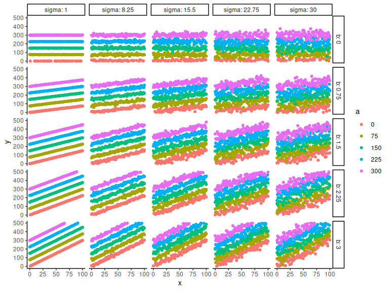
Hopefully its clear that the a parameter is the intersection i.e. the y-value when x = 0. The parameter b represents the slope of the line, higher b, steeper lines. Lastly sigma represents the spread of data points, higher values represents greater spread.

Psychometric functions.

Now we do the same for a psychometric function to take an example a bit less known. The psychometric function is a function that maps continuous values ] $-\infty$ ; $\infty$ [ to probabilities [0 ; 1].

The most common function to use is the cumulative normal distribution or the probit model with the functional form:

$p_i = 0.5 + 0.5 \cdot erf\left(\frac{x_i - \alpha }{\beta \cdot \sqrt{2}}\right)$

Here $p_i$ represents the probability of answering 1, and x represents the independent variable that when increases increases the probability of responding 1.

In the same vain as with the normal distribution we simulate probabilities, from simulated values of the parameters ( $\alpha$ & $\beta$ ) and the independent variable $x_i$ .

#data points
N = 100
#threshold
alpha = 10
#slope
beta = 3
#x's
x = seq(0,30, length.out = N)

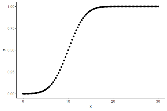
We can then obtain the probabilities by writing the formula:

# getting the probabilities from the model and the parameters
p = 0.5+0.5*pracma::erf((x-alpha)/(sqrt(2)*beta))

Now importantly we can plot it ensuring ourselves that it makes sense

data.frame() %>% ggplot(aes(x =x,y = p))+geom_point()+theme_classic()

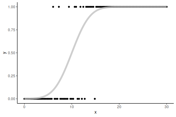
The additional thing here is that we do not observe these probabilities, but the realization of these (i.e. the actual binary responses that come from these probabilities). In order to simulate this we need another probability density function (just as we used the normal distribution to get noise about our y_i’s) here the binominal distribution which converts probabilities to binary responses $y_i$ :

# generating binary responses from the probabilities above
y = rbinom(N,1,p)

We can then plot the binary realization of the probabilities as well as the curve from above:

data.frame() %>% 
  ggplot(aes(x =x,y = y))+
  geom_point()+
  theme_classic()+
  geom_line(aes(x = x, y = p), col = "grey", alpha = 0.75, linewidth = 2)

Now we can again fit this using normal linear modeling.

This would be done by with the following code:

# fittiing the model using generalized linear model and plotting as a table
m1 = glm(y ~ x, family = binomial(link = "probit"))
summary(m1)

## 
## Call:
## glm(formula = y ~ x, family = binomial(link = "probit"))
## 
## Coefficients:
##             Estimate Std. Error z value Pr(>|z|)    
## (Intercept) -3.35084    0.72546  -4.619 3.86e-06 ***
## x            0.30516    0.06272   4.866 1.14e-06 ***
## ---
## Signif. codes:  0 '***' 0.001 '**' 0.01 '*' 0.05 '.' 0.1 ' ' 1
## 
## (Dispersion parameter for binomial family taken to be 1)
## 
##     Null deviance: 131.791  on 99  degrees of freedom
## Residual deviance:  39.341  on 98  degrees of freedom
## AIC: 43.341
## 
## Number of Fisher Scoring iterations: 8

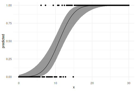
As can be seen the output is quite different which relates to the how the model is specified, this is beyond the scope of this Markdown, but it suffices to plot the outcome of the model and indeed show its the same as out simulation:

# Plotting the marginal effects of the model
effects = ggpredict(m1,terms = "x [all]")



# the plot below is commented out as it does not knit (I do not know why)

data.frame(effects) %>%
  ggplot(aes(x = x, y = predicted))+
  geom_line()+geom_ribbon(aes(ymin = conf.low, ymax = conf.high), alpha = 0.5)+
  geom_point(data = data.frame(x =x,y = y), aes(x = x ,y = y))+
  theme_minimal()

Generalized simulations (psychometric functions).

Now we can do the same step as we did with the linear model of plotting many different combinations of parameters values of the function. Before doing this we introduce a third parameter of the psychometric, which means that the functional relationship between our independent variable $x_i$ and the probability $p_i$ is now:

$p_i = \lambda + (1-2*\lambda) * \left(0.5 + 0.5 \cdot erf\left(\frac{x_i - \alpha }{\beta \cdot \sqrt{2}}\right)\right)$

The 3 parameters $\lambda$ , $\alpha$ , $\beta$ are called lapse rate, threshold and slope respectively. This hopefully becomes clear below.

# keep the number of data points constant (could also vary this)
N = 200
#intercept
alpha = seq(0,20,length.out = 5)
#slope
beta = seq(1,10,length.out = 5)
#sigma
lambda = seq(0,0.3,length.out = 5)

parameters = expand.grid(alpha = alpha,
                         beta = beta,
                         lambda = lambda,
                         N = N)

#lastly we put it together in a dataframe:
df = parameters %>% rowwise() %>% 
  mutate(x = list(seq(-10,30, length.out = N))) %>% 
  unnest(x)

Now we calculate the latent (unobserved) probability, $p_i$ .

# define function based on functional relationship
psycho = function(x,alpha,beta,lambda){
  return(lambda + (1-2*lambda) * (0.5+0.5*pracma::erf((x-alpha)/(beta*sqrt(2)))))
}
# getting the p_i and afterwards geting the binary responses based on p
df = df %>% 
  mutate(p = psycho(x,alpha,beta,lambda)) %>% 
  mutate(y = rbinom(n(),1,p))

And we can then plot the different combinations (here we plot the probabilities) as the binary responses gets messy.

df %>% 
  # Make parameters factors
  mutate(alpha = as.factor(alpha), beta = as.factor(beta), lambda = as.factor(lambda)) %>% 
  # ggplot
  ggplot(aes(x = x, y = p, col = alpha))+
  # scale the y axiis
  scale_y_continuous(limits = c(0,1))+
  # Gris the lapse and the slope
  facet_grid(beta~lambda, scales = "free", labeller = label_both)+
  # draw the lines
  geom_line(linewidth = 1.2)+theme_classic()

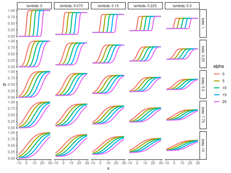
Hopefully its clear that the $\alpha$ parameter is the x-value where the probability is 0.5 i.e. the x-value when y = 0. The parameter $\beta$ represents the slope of the line, higher b less steep lines.

Lastly $\lambda$ represents the lapse rate and governs where the function starts and ends. i.e. when x -> $-\infty$ y -> $\lambda$ and when x -> $\infty$ y -> $1-\lambda$ .

Final remarks.

This finishes the section on data simulation with two simple models.

The main takeaway from this markdown should be that making the assumptions of the model explicit is relatively easy, and will be worthwhile when building the model in Stan later.

Understanding what the free parameters of the model mean and what values are sensible for your problem is vital to the further steps.

Share on

X (formerly Twitter) Facebook LinkedIn

Jesper Fischer Ehmsen

Data Simulation

Table of content

Overview.

Simulation (Linear model).

Generalized simulations (linear model).

Psychometric functions.

Generalized simulations (psychometric functions).

Final remarks.

Share on

You May Also Enjoy

Multivariate Priors And Correlations

Distributions

Parameter Recovery

Hierarchical Models