
Diagnostics
Published:
- Bayesian Workflow
This R markdown document is an introduction of how to diagnose Stan models.
Table of content
Overview.
When fitting models in Stan we have to ensure that the sampling process of the joint posterior distribution goes smoothly. If Stan encounters errors, or trouble in the sampling process then the estimates of the model cannot be trusted and diagnosing the model is vital for further development. My general heuristic for what might go wrong is in the following order:
- Coding error
- Missing priors
- Constrained parameters (that haven’t been constrained)
- parameterization
Before diving into the types of errors and warning Stan produces we first need to examine the types of problems we might face;
Generally to trust the sampler’s results we need to achieve no divergences and good mixing of the chains, which will have Rhat values close to 1 for each of our parameters. Generally the max_treedepth argument is harmless by itself, but will speak to the fact that there might be something wrong in the model.
To look at these diagnostics in pratice we need a degenerate model. To do this we simulate data as before, but with a coding error in the stan model:
#data points
N = 100
#intercept
a = 10
#slope
b = 3
#sigma
sigma = 20
#x's
x = seq(0,100, length.out = N)
#y's
y = rnorm(N,a+b*x,sigma)
//This block defines the input that. So these things needs to go into the model
data {
  //Define the number of datapoints this is defined by an integer
  int N;
  //Define a vector called y that is as long as the number of datapoints (i.e. N)
  vector[N] y;
  // same as y but a variable called x our independent variable
  vector[N] x;
}

// This is the parameters block. Here we define the free parameters
// which are the onces that STAN estimates for us.
// this is again a,b and sigma
parameters {
  real a;
  real b;
  real sigma;
}

// This is the model block here we define how we believe the model is
// (of cause we simulated the data so we just put in the same thing as we did when simulating)

model {
  y ~ normal(a+x, sigma);
}
Note this is the same model as in “Model fitting to simulated data markdown”, where a coding error has been introduced (the missing “b” in the model block). Also note here no priors have been specified, this will be important later!
# Fit the STAN model
fit = model_obj2$sample(data = list(N =N, x = x, y =y), seed = seeds)
## Running MCMC with 4 sequential chains...
##
## Chain 1 Iteration:    1 / 2000 [  0%]  (Warmup)
## Chain 1 Iteration:  100 / 2000 [  5%]  (Warmup)

## Chain 1 Informational Message: The current Metropolis proposal is about to be rejected because of the following issue:

## Chain 1 Exception: normal_lpdf: Scale parameter is -416.238, but must be positive! (in '/tmp/RtmpLT7ubk/model-1f026ea79b6a.stan', line 23, column 2 to column 25)

## Chain 1 If this warning occurs sporadically, such as for highly constrained variable types like covariance matrices, then the sampler is fine,

## Chain 1 but if this warning occurs often then your model may be either severely ill-conditioned or misspecified.

## Chain 1

## Chain 1 Informational Message: The current Metropolis proposal is about to be rejected because of the following issue:

## Chain 1 Exception: normal_lpdf: Scale parameter is -79.6013, but must be positive! (in '/tmp/RtmpLT7ubk/model-1f026ea79b6a.stan', line 23, column 2 to column 25)

## Chain 1 If this warning occurs sporadically, such as for highly constrained variable types like covariance matrices, then the sampler is fine,

## Chain 1 but if this warning occurs often then your model may be either severely ill-conditioned or misspecified.

## Chain 1

## Chain 1 Iteration:  200 / 2000 [ 10%]  (Warmup)
## Chain 1 Iteration:  300 / 2000 [ 15%]  (Warmup)
## Chain 1 Iteration:  400 / 2000 [ 20%]  (Warmup)
## Chain 1 Iteration:  500 / 2000 [ 25%]  (Warmup)
## Chain 1 Iteration:  600 / 2000 [ 30%]  (Warmup)
## Chain 1 Iteration:  700 / 2000 [ 35%]  (Warmup)

## Chain 1 Informational Message: The current Metropolis proposal is about to be rejected because of the following issue:

## Chain 1 Exception: normal_lpdf: Scale parameter is -216.94, but must be positive! (in '/tmp/RtmpLT7ubk/model-1f026ea79b6a.stan', line 23, column 2 to column 25)

## Chain 1 If this warning occurs sporadically, such as for highly constrained variable types like covariance matrices, then the sampler is fine,

## Chain 1 but if this warning occurs often then your model may be either severely ill-conditioned or misspecified.

## Chain 1

## Chain 1 Informational Message: The current Metropolis proposal is about to be rejected because of the following issue:

## Chain 1 Exception: normal_lpdf: Scale parameter is -49.3037, but must be positive! (in '/tmp/RtmpLT7ubk/model-1f026ea79b6a.stan', line 23, column 2 to column 25)

## Chain 1 If this warning occurs sporadically, such as for highly constrained variable types like covariance matrices, then the sampler is fine,

## Chain 1 but if this warning occurs often then your model may be either severely ill-conditioned or misspecified.

## Chain 1

## Chain 1 Iteration:  800 / 2000 [ 40%]  (Warmup)
## Chain 1 Iteration:  900 / 2000 [ 45%]  (Warmup)

## Chain 1 Informational Message: The current Metropolis proposal is about to be rejected because of the following issue:

## Chain 1 Exception: normal_lpdf: Scale parameter is -70.4325, but must be positive! (in '/tmp/RtmpLT7ubk/model-1f026ea79b6a.stan', line 23, column 2 to column 25)

## Chain 1 If this warning occurs sporadically, such as for highly constrained variable types like covariance matrices, then the sampler is fine,

## Chain 1 but if this warning occurs often then your model may be either severely ill-conditioned or misspecified.

## Chain 1

## Chain 1 Iteration: 1000 / 2000 [ 50%]  (Warmup)
## Chain 1 Iteration: 1001 / 2000 [ 50%]  (Sampling)
## Chain 1 Iteration: 1100 / 2000 [ 55%]  (Sampling)
## Chain 1 Iteration: 1200 / 2000 [ 60%]  (Sampling)
## Chain 1 Iteration: 1300 / 2000 [ 65%]  (Sampling)
## Chain 1 Iteration: 1400 / 2000 [ 70%]  (Sampling)
## Chain 1 Iteration: 1500 / 2000 [ 75%]  (Sampling)
## Chain 1 Iteration: 1600 / 2000 [ 80%]  (Sampling)
## Chain 1 Iteration: 1700 / 2000 [ 85%]  (Sampling)
## Chain 1 Iteration: 1800 / 2000 [ 90%]  (Sampling)
## Chain 1 Iteration: 1900 / 2000 [ 95%]  (Sampling)
## Chain 1 Iteration: 2000 / 2000 [100%]  (Sampling)
## Chain 1 finished in 1.5 seconds.
## Chain 2 Iteration:    1 / 2000 [  0%]  (Warmup)
## Chain 2 Iteration:  100 / 2000 [  5%]  (Warmup)
## Chain 2 Iteration:  200 / 2000 [ 10%]  (Warmup)
## Chain 2 Iteration:  300 / 2000 [ 15%]  (Warmup)
## Chain 2 Iteration:  400 / 2000 [ 20%]  (Warmup)
## Chain 2 Iteration:  500 / 2000 [ 25%]  (Warmup)

## Chain 2 Informational Message: The current Metropolis proposal is about to be rejected because of the following issue:

## Chain 2 Exception: normal_lpdf: Scale parameter is -89.4157, but must be positive! (in '/tmp/RtmpLT7ubk/model-1f026ea79b6a.stan', line 23, column 2 to column 25)

## Chain 2 If this warning occurs sporadically, such as for highly constrained variable types like covariance matrices, then the sampler is fine,

## Chain 2 but if this warning occurs often then your model may be either severely ill-conditioned or misspecified.

## Chain 2

## Chain 2 Iteration:  600 / 2000 [ 30%]  (Warmup)
## Chain 2 Iteration:  700 / 2000 [ 35%]  (Warmup)
## Chain 2 Iteration:  800 / 2000 [ 40%]  (Warmup)
## Chain 2 Iteration:  900 / 2000 [ 45%]  (Warmup)

## Chain 2 Informational Message: The current Metropolis proposal is about to be rejected because of the following issue:

## Chain 2 Exception: normal_lpdf: Scale parameter is -72.0136, but must be positive! (in '/tmp/RtmpLT7ubk/model-1f026ea79b6a.stan', line 23, column 2 to column 25)

## Chain 2 If this warning occurs sporadically, such as for highly constrained variable types like covariance matrices, then the sampler is fine,

## Chain 2 but if this warning occurs often then your model may be either severely ill-conditioned or misspecified.

## Chain 2

## Chain 2 Iteration: 1000 / 2000 [ 50%]  (Warmup)
## Chain 2 Iteration: 1001 / 2000 [ 50%]  (Sampling)
## Chain 2 Iteration: 1100 / 2000 [ 55%]  (Sampling)
## Chain 2 Iteration: 1200 / 2000 [ 60%]  (Sampling)
## Chain 2 Iteration: 1300 / 2000 [ 65%]  (Sampling)
## Chain 2 Iteration: 1400 / 2000 [ 70%]  (Sampling)
## Chain 2 Iteration: 1500 / 2000 [ 75%]  (Sampling)
## Chain 2 Iteration: 1600 / 2000 [ 80%]  (Sampling)
## Chain 2 Iteration: 1700 / 2000 [ 85%]  (Sampling)
## Chain 2 Iteration: 1800 / 2000 [ 90%]  (Sampling)
## Chain 2 Iteration: 1900 / 2000 [ 95%]  (Sampling)
## Chain 2 Iteration: 2000 / 2000 [100%]  (Sampling)
## Chain 2 finished in 1.5 seconds.
## Chain 3 Iteration:    1 / 2000 [  0%]  (Warmup)
## Chain 3 Iteration:  100 / 2000 [  5%]  (Warmup)

## Chain 3 Informational Message: The current Metropolis proposal is about to be rejected because of the following issue:

## Chain 3 Exception: normal_lpdf: Scale parameter is -106.375, but must be positive! (in '/tmp/RtmpLT7ubk/model-1f026ea79b6a.stan', line 23, column 2 to column 25)

## Chain 3 If this warning occurs sporadically, such as for highly constrained variable types like covariance matrices, then the sampler is fine,

## Chain 3 but if this warning occurs often then your model may be either severely ill-conditioned or misspecified.

## Chain 3

## Chain 3 Informational Message: The current Metropolis proposal is about to be rejected because of the following issue:

## Chain 3 Exception: normal_lpdf: Scale parameter is -6.42058, but must be positive! (in '/tmp/RtmpLT7ubk/model-1f026ea79b6a.stan', line 23, column 2 to column 25)

## Chain 3 If this warning occurs sporadically, such as for highly constrained variable types like covariance matrices, then the sampler is fine,

## Chain 3 but if this warning occurs often then your model may be either severely ill-conditioned or misspecified.

## Chain 3

## Chain 3 Iteration:  200 / 2000 [ 10%]  (Warmup)
## Chain 3 Iteration:  300 / 2000 [ 15%]  (Warmup)

## Chain 3 Informational Message: The current Metropolis proposal is about to be rejected because of the following issue:

## Chain 3 Exception: normal_lpdf: Scale parameter is -236.066, but must be positive! (in '/tmp/RtmpLT7ubk/model-1f026ea79b6a.stan', line 23, column 2 to column 25)

## Chain 3 If this warning occurs sporadically, such as for highly constrained variable types like covariance matrices, then the sampler is fine,

## Chain 3 but if this warning occurs often then your model may be either severely ill-conditioned or misspecified.

## Chain 3

## Chain 3 Iteration:  400 / 2000 [ 20%]  (Warmup)
## Chain 3 Iteration:  500 / 2000 [ 25%]  (Warmup)

## Chain 3 Informational Message: The current Metropolis proposal is about to be rejected because of the following issue:

## Chain 3 Exception: normal_lpdf: Scale parameter is -57.3216, but must be positive! (in '/tmp/RtmpLT7ubk/model-1f026ea79b6a.stan', line 23, column 2 to column 25)

## Chain 3 If this warning occurs sporadically, such as for highly constrained variable types like covariance matrices, then the sampler is fine,

## Chain 3 but if this warning occurs often then your model may be either severely ill-conditioned or misspecified.

## Chain 3

## Chain 3 Iteration:  600 / 2000 [ 30%]  (Warmup)
## Chain 3 Iteration:  700 / 2000 [ 35%]  (Warmup)
## Chain 3 Iteration:  800 / 2000 [ 40%]  (Warmup)
## Chain 3 Iteration:  900 / 2000 [ 45%]  (Warmup)
## Chain 3 Iteration: 1000 / 2000 [ 50%]  (Warmup)
## Chain 3 Iteration: 1001 / 2000 [ 50%]  (Sampling)
## Chain 3 Iteration: 1100 / 2000 [ 55%]  (Sampling)
## Chain 3 Iteration: 1200 / 2000 [ 60%]  (Sampling)
## Chain 3 Iteration: 1300 / 2000 [ 65%]  (Sampling)
## Chain 3 Iteration: 1400 / 2000 [ 70%]  (Sampling)
## Chain 3 Iteration: 1500 / 2000 [ 75%]  (Sampling)
## Chain 3 Iteration: 1600 / 2000 [ 80%]  (Sampling)
## Chain 3 Iteration: 1700 / 2000 [ 85%]  (Sampling)
## Chain 3 Iteration: 1800 / 2000 [ 90%]  (Sampling)
## Chain 3 Iteration: 1900 / 2000 [ 95%]  (Sampling)
## Chain 3 Iteration: 2000 / 2000 [100%]  (Sampling)
## Chain 3 finished in 1.7 seconds.

## Chain 4 Rejecting initial value:

## Chain 4   Error evaluating the log probability at the initial value.

## Chain 4 Exception: normal_lpdf: Scale parameter is -0.650394, but must be positive! (in '/tmp/RtmpLT7ubk/model-1f026ea79b6a.stan', line 23, column 2 to column 25)
## Chain 4 Exception: normal_lpdf: Scale parameter is -0.650394, but must be positive! (in '/tmp/RtmpLT7ubk/model-1f026ea79b6a.stan', line 23, column 2 to column 25)

## Chain 4 Iteration:    1 / 2000 [  0%]  (Warmup)
## Chain 4 Iteration:  100 / 2000 [  5%]  (Warmup)

## Chain 4 Informational Message: The current Metropolis proposal is about to be rejected because of the following issue:

## Chain 4 Exception: normal_lpdf: Scale parameter is -56.5163, but must be positive! (in '/tmp/RtmpLT7ubk/model-1f026ea79b6a.stan', line 23, column 2 to column 25)

## Chain 4 If this warning occurs sporadically, such as for highly constrained variable types like covariance matrices, then the sampler is fine,

## Chain 4 but if this warning occurs often then your model may be either severely ill-conditioned or misspecified.

## Chain 4

## Chain 4 Iteration:  200 / 2000 [ 10%]  (Warmup)
## Chain 4 Iteration:  300 / 2000 [ 15%]  (Warmup)

## Chain 4 Informational Message: The current Metropolis proposal is about to be rejected because of the following issue:

## Chain 4 Exception: normal_lpdf: Scale parameter is -86.315, but must be positive! (in '/tmp/RtmpLT7ubk/model-1f026ea79b6a.stan', line 23, column 2 to column 25)

## Chain 4 If this warning occurs sporadically, such as for highly constrained variable types like covariance matrices, then the sampler is fine,

## Chain 4 but if this warning occurs often then your model may be either severely ill-conditioned or misspecified.

## Chain 4

## Chain 4 Iteration:  400 / 2000 [ 20%]  (Warmup)
## Chain 4 Iteration:  500 / 2000 [ 25%]  (Warmup)

## Chain 4 Informational Message: The current Metropolis proposal is about to be rejected because of the following issue:

## Chain 4 Exception: normal_lpdf: Scale parameter is -77.1527, but must be positive! (in '/tmp/RtmpLT7ubk/model-1f026ea79b6a.stan', line 23, column 2 to column 25)

## Chain 4 If this warning occurs sporadically, such as for highly constrained variable types like covariance matrices, then the sampler is fine,

## Chain 4 but if this warning occurs often then your model may be either severely ill-conditioned or misspecified.

## Chain 4

## Chain 4 Iteration:  600 / 2000 [ 30%]  (Warmup)
## Chain 4 Iteration:  700 / 2000 [ 35%]  (Warmup)
## Chain 4 Iteration:  800 / 2000 [ 40%]  (Warmup)
## Chain 4 Iteration:  900 / 2000 [ 45%]  (Warmup)
## Chain 4 Iteration: 1000 / 2000 [ 50%]  (Warmup)
## Chain 4 Iteration: 1001 / 2000 [ 50%]  (Sampling)
## Chain 4 Iteration: 1100 / 2000 [ 55%]  (Sampling)
## Chain 4 Iteration: 1200 / 2000 [ 60%]  (Sampling)
## Chain 4 Iteration: 1300 / 2000 [ 65%]  (Sampling)
## Chain 4 Iteration: 1400 / 2000 [ 70%]  (Sampling)
## Chain 4 Iteration: 1500 / 2000 [ 75%]  (Sampling)
## Chain 4 Iteration: 1600 / 2000 [ 80%]  (Sampling)
## Chain 4 Iteration: 1700 / 2000 [ 85%]  (Sampling)
## Chain 4 Iteration: 1800 / 2000 [ 90%]  (Sampling)
## Chain 4 Iteration: 1900 / 2000 [ 95%]  (Sampling)
## Chain 4 Iteration: 2000 / 2000 [100%]  (Sampling)
## Chain 4 finished in 1.6 seconds.
##
## All 4 chains finished successfully.
## Mean chain execution time: 1.6 seconds.
## Total execution time: 6.7 seconds.

## Warning: 1579 of 4000 (39.0%) transitions hit the maximum treedepth limit of 10.
## See https://mc-stan.org/misc/warnings for details.
Here we run into our first real warning; the sampler hitting the maximum tree depth limit. Opening the model summary we can immediately see the issue.
# calling the fitted object
fit
##  variable          mean        median           sd          mad            q5
##     lp__  -4.644500e+02 -4.641200e+02 1.020000e+00 7.100000e-01 -4.665300e+02
##     a      1.119200e+02  1.119100e+02 6.260000e+00 6.150000e+00  1.017800e+02
##     b     -8.309004e+19 -2.914865e+19 4.289424e+20 3.114152e+20 -1.030944e+21
##     sigma  6.358000e+01  6.326000e+01 4.660000e+00 4.620000e+00  5.658000e+01
##            q95 rhat ess_bulk ess_tail
##  -4.634800e+02 1.00     1879     2354
##   1.221200e+02 1.00     3934     3029
##   4.698208e+20 2.73        4       11
##   7.163000e+01 1.00     3358     2568
The estimates for our slope parameter “b” is ridiculously high. This is usually because no prior has been set on the parameter and the parameter is not “used” by the model. Another thing to note in the summary statistics is the three last columns “Rhat”, “ess_bulk” and “ess_tail”. These values indicate how well the resulting chains have merged together. Generally we want rhat values to be very close to 1 (0.99 ; 1.03) and the ess_bulk and ess_tail values to be as high as possible, but generally higher than 200 / 400. We see from the summary statistics that only the b-parameter is having trouble with these diagnostics. All three diagnostics (rhat, ess_bulk and ess_tail) are related to how well the chains of the sampler have converged to a single posterior distribution which leads us to trace-plots.
Trace plots
Trace plots are plots of the sampled values from Stan on each iteration of the sampling. In these trace-plots we plot each iteration on the x-axis and on the y-axis we plot the sampled parameter value. What we want to see is that all of the chains we run are “mixing” together such that we can faithfully average across them. This also entails that there is no drift in the chains (i.e. moving up or down as iterations increase). As an aside because I have not yet mentioned the sampler parameters, Stan as per default runs 4 chains, 1000 warm-up samples (thrown away for inference) and 1000 samples. This is all the output that happens when fitting the model.
# calling the mcmc_trace function on the draws of the three parameters
mcmc_trace(fit$draws(c("a","b","sigma")))
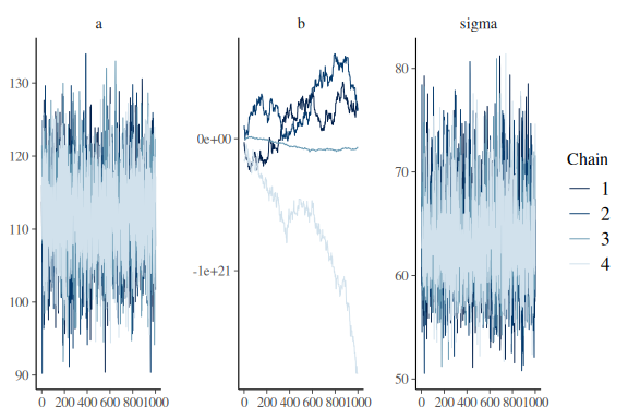
As can be seen in the traceplots the slope parameter has chains that do not mix, whereas the plots for a and sigma are great. What one looks for is that its practically impossible to distinguish the chains (colors). Good mixing chains look like hairy caterpillars.
Next we try the same model as above but putting the prior we used in the “prior markdown” on the parameters.
//This block defines the input that. So these things needs to go into the model
data {
  //Define the number of datapoints this is defined by an integer
  int N;
  //Define a vector called y that is as long as the number of datapoints (i.e. N)
  vector[N] y;
  // same as y but a variable called x our independent variable
  vector[N] x;
}

// This is the parameters block. Here we define the free parameters
// which are the onces that STAN estimates for us.
// this is again a,b and sigma
parameters {
  real a;
  real b;
  real sigma;
}

// This is the model block here we define the model

model {
  a ~ normal(0,20);
  b ~ normal(0,3);
  //Note the prior for sigma is exponentiated to keep it positive
  sigma ~ normal(0,1);

  y ~ normal(a+x, exp(sigma));
}
# Fit the STAN model

fit = model_obj2$sample(data = list(N =N, x = x, y =y), seed = seeds)
## Running MCMC with 4 sequential chains...
##
## Chain 1 Iteration:    1 / 2000 [  0%]  (Warmup)
## Chain 1 Iteration:  100 / 2000 [  5%]  (Warmup)
## Chain 1 Iteration:  200 / 2000 [ 10%]  (Warmup)
## Chain 1 Iteration:  300 / 2000 [ 15%]  (Warmup)
## Chain 1 Iteration:  400 / 2000 [ 20%]  (Warmup)
## Chain 1 Iteration:  500 / 2000 [ 25%]  (Warmup)
## Chain 1 Iteration:  600 / 2000 [ 30%]  (Warmup)
## Chain 1 Iteration:  700 / 2000 [ 35%]  (Warmup)
## Chain 1 Iteration:  800 / 2000 [ 40%]  (Warmup)
## Chain 1 Iteration:  900 / 2000 [ 45%]  (Warmup)
## Chain 1 Iteration: 1000 / 2000 [ 50%]  (Warmup)
## Chain 1 Iteration: 1001 / 2000 [ 50%]  (Sampling)
## Chain 1 Iteration: 1100 / 2000 [ 55%]  (Sampling)
## Chain 1 Iteration: 1200 / 2000 [ 60%]  (Sampling)
## Chain 1 Iteration: 1300 / 2000 [ 65%]  (Sampling)
## Chain 1 Iteration: 1400 / 2000 [ 70%]  (Sampling)
## Chain 1 Iteration: 1500 / 2000 [ 75%]  (Sampling)
## Chain 1 Iteration: 1600 / 2000 [ 80%]  (Sampling)
## Chain 1 Iteration: 1700 / 2000 [ 85%]  (Sampling)
## Chain 1 Iteration: 1800 / 2000 [ 90%]  (Sampling)
## Chain 1 Iteration: 1900 / 2000 [ 95%]  (Sampling)
## Chain 1 Iteration: 2000 / 2000 [100%]  (Sampling)
## Chain 1 finished in 0.1 seconds.
## Chain 2 Iteration:    1 / 2000 [  0%]  (Warmup)
## Chain 2 Iteration:  100 / 2000 [  5%]  (Warmup)
## Chain 2 Iteration:  200 / 2000 [ 10%]  (Warmup)
## Chain 2 Iteration:  300 / 2000 [ 15%]  (Warmup)
## Chain 2 Iteration:  400 / 2000 [ 20%]  (Warmup)
## Chain 2 Iteration:  500 / 2000 [ 25%]  (Warmup)
## Chain 2 Iteration:  600 / 2000 [ 30%]  (Warmup)
## Chain 2 Iteration:  700 / 2000 [ 35%]  (Warmup)
## Chain 2 Iteration:  800 / 2000 [ 40%]  (Warmup)
## Chain 2 Iteration:  900 / 2000 [ 45%]  (Warmup)
## Chain 2 Iteration: 1000 / 2000 [ 50%]  (Warmup)
## Chain 2 Iteration: 1001 / 2000 [ 50%]  (Sampling)
## Chain 2 Iteration: 1100 / 2000 [ 55%]  (Sampling)
## Chain 2 Iteration: 1200 / 2000 [ 60%]  (Sampling)
## Chain 2 Iteration: 1300 / 2000 [ 65%]  (Sampling)
## Chain 2 Iteration: 1400 / 2000 [ 70%]  (Sampling)
## Chain 2 Iteration: 1500 / 2000 [ 75%]  (Sampling)
## Chain 2 Iteration: 1600 / 2000 [ 80%]  (Sampling)
## Chain 2 Iteration: 1700 / 2000 [ 85%]  (Sampling)
## Chain 2 Iteration: 1800 / 2000 [ 90%]  (Sampling)
## Chain 2 Iteration: 1900 / 2000 [ 95%]  (Sampling)
## Chain 2 Iteration: 2000 / 2000 [100%]  (Sampling)
## Chain 2 finished in 0.1 seconds.
## Chain 3 Iteration:    1 / 2000 [  0%]  (Warmup)
## Chain 3 Iteration:  100 / 2000 [  5%]  (Warmup)
## Chain 3 Iteration:  200 / 2000 [ 10%]  (Warmup)
## Chain 3 Iteration:  300 / 2000 [ 15%]  (Warmup)
## Chain 3 Iteration:  400 / 2000 [ 20%]  (Warmup)
## Chain 3 Iteration:  500 / 2000 [ 25%]  (Warmup)
## Chain 3 Iteration:  600 / 2000 [ 30%]  (Warmup)
## Chain 3 Iteration:  700 / 2000 [ 35%]  (Warmup)
## Chain 3 Iteration:  800 / 2000 [ 40%]  (Warmup)
## Chain 3 Iteration:  900 / 2000 [ 45%]  (Warmup)
## Chain 3 Iteration: 1000 / 2000 [ 50%]  (Warmup)
## Chain 3 Iteration: 1001 / 2000 [ 50%]  (Sampling)
## Chain 3 Iteration: 1100 / 2000 [ 55%]  (Sampling)
## Chain 3 Iteration: 1200 / 2000 [ 60%]  (Sampling)
## Chain 3 Iteration: 1300 / 2000 [ 65%]  (Sampling)
## Chain 3 Iteration: 1400 / 2000 [ 70%]  (Sampling)
## Chain 3 Iteration: 1500 / 2000 [ 75%]  (Sampling)
## Chain 3 Iteration: 1600 / 2000 [ 80%]  (Sampling)
## Chain 3 Iteration: 1700 / 2000 [ 85%]  (Sampling)
## Chain 3 Iteration: 1800 / 2000 [ 90%]  (Sampling)
## Chain 3 Iteration: 1900 / 2000 [ 95%]  (Sampling)
## Chain 3 Iteration: 2000 / 2000 [100%]  (Sampling)
## Chain 3 finished in 0.1 seconds.
## Chain 4 Iteration:    1 / 2000 [  0%]  (Warmup)
## Chain 4 Iteration:  100 / 2000 [  5%]  (Warmup)
## Chain 4 Iteration:  200 / 2000 [ 10%]  (Warmup)
## Chain 4 Iteration:  300 / 2000 [ 15%]  (Warmup)
## Chain 4 Iteration:  400 / 2000 [ 20%]  (Warmup)
## Chain 4 Iteration:  500 / 2000 [ 25%]  (Warmup)
## Chain 4 Iteration:  600 / 2000 [ 30%]  (Warmup)
## Chain 4 Iteration:  700 / 2000 [ 35%]  (Warmup)
## Chain 4 Iteration:  800 / 2000 [ 40%]  (Warmup)
## Chain 4 Iteration:  900 / 2000 [ 45%]  (Warmup)
## Chain 4 Iteration: 1000 / 2000 [ 50%]  (Warmup)
## Chain 4 Iteration: 1001 / 2000 [ 50%]  (Sampling)
## Chain 4 Iteration: 1100 / 2000 [ 55%]  (Sampling)
## Chain 4 Iteration: 1200 / 2000 [ 60%]  (Sampling)
## Chain 4 Iteration: 1300 / 2000 [ 65%]  (Sampling)
## Chain 4 Iteration: 1400 / 2000 [ 70%]  (Sampling)
## Chain 4 Iteration: 1500 / 2000 [ 75%]  (Sampling)
## Chain 4 Iteration: 1600 / 2000 [ 80%]  (Sampling)
## Chain 4 Iteration: 1700 / 2000 [ 85%]  (Sampling)
## Chain 4 Iteration: 1800 / 2000 [ 90%]  (Sampling)
## Chain 4 Iteration: 1900 / 2000 [ 95%]  (Sampling)
## Chain 4 Iteration: 2000 / 2000 [100%]  (Sampling)
## Chain 4 finished in 0.0 seconds.
##
## All 4 chains finished successfully.
## Mean chain execution time: 0.1 seconds.
## Total execution time: 0.6 seconds.
Now there is no apparent issue from the sampler.
# calling the fitted object

fit
##  variable    mean  median   sd  mad      q5     q95 rhat ess_bulk ess_tail
##     lp__  -487.74 -487.41 1.24 1.03 -490.26 -486.39 1.00     2041     2586
##     a      101.71  101.85 6.23 6.07   91.24  111.83 1.00     3134     2780
##     b       -0.01    0.02 2.98 2.97   -4.95    4.79 1.00     3479     2938
##     sigma    4.14    4.13 0.07 0.07    4.02    4.26 1.00     3855     3089
And we see that the slope parameter from the stan summary statistics is exactly the prior that was put in; a mean of 0 and a standard deviation of 3.
Furthermore we see that the Rhat, ess_bulk, ess_tail look much better. We can also plot the traceplots again:
# calling the mcmc_trace function on the draws of the three parameters

mcmc_trace(fit$draws(c("a","b","sigma")))
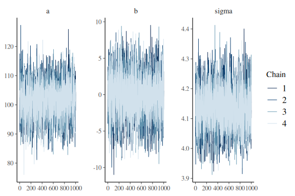
looks perfectly fine now.
Now we have avoided the sampler issues by including priors. But remember this was a miss-specified model and just using the sampler diagnostics, when we include priors, we do not find the miss-specification. This is why prior-posterior updates and posterior predictive checks are vital.
Investigating the posteriors
Prior posterior updates. Next we plot the prior-posterior update, as in the “priors markdown”.
# we row-bind two dataframe together here firstly the draws
# from the stan-model (the posterior distribution for each parameter)
rbind(
  as_draws_df(fit$draws(c("a","b","sigma"))) %>%
    select(-contains(".")) %>% pivot_longer(everything()) %>%
    mutate(pp = "Posterior"),
# Secondly we row-bind what the priors of each of
# the parameters were (these are the same distributions and values in the STAN code)
  data.frame(name = rep(c("a","b","sigma"), each = 4000),
             value = c(rnorm(4000,0,20),rnorm(4000,0,3),exp(rnorm(4000,0,1)))) %>%
    mutate(pp = "Prior")
  ) %>%
#And lastly we plot the prior and posterior together
  ggplot(aes(x = value, fill = pp))+
  geom_histogram(col = "black", position = "identity", alpha = 0.5)+
  facet_wrap(~name, scales = "free")+
  theme_minimal()
## Warning: Dropping 'draws_df' class as required metadata was removed.

## `stat_bin()` using `bins = 30`. Pick better value with `binwidth`.
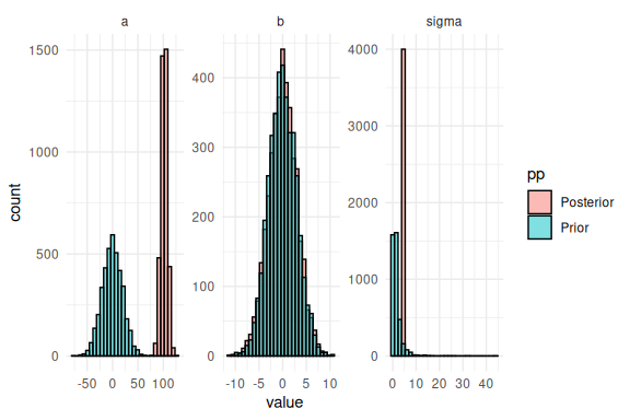
Here we see that something is not right. For the b-parameter the prior is excatly identical to the posterior, which indicates that we forgot to use that parameter in our model. Due to misspecification the other parameters a and compensate and are now quite outside the range of what was simulated (mostly a).
Posterior predictive checks:
# number of draws to plot
n_draws_plot = 100

# the id's of the 100 draws
draw_id = sample(1:4000,n_draws_plot)

# getting the posterior distribution for each of the parameters
# and then adding the x-values (here just a sequence of numbers from 0 to 100)
as_draws_df(fit$draws(c("a","b","sigma"))) %>%
  select(-contains(".")) %>% mutate(draw = 1:n(),
                                    x = list(seq(0,100, length.out = N))) %>%
# select the draws we want to plot
  filter(draw %in% draw_id) %>%
# make the x's into a rowwise dataframe
  unnest((x)) %>%
# calculate the model predicitions from each of our estimated draws of the parameters
  mutate(y_pred = rnorm(n(),a+b*x,exp(sigma))) %>%
# plot the resuls
  ggplot()+
  geom_line(aes(x = y_pred, group = draw), col = "black", alpha = 0.5, stat = "density")+
  geom_histogram(data = data.frame(y = y),aes(x = y, after_stat(density)),col = "black", fill = "red")+
  theme_minimal()
## Warning: Dropping 'draws_df' class as required metadata was removed.

## `stat_bin()` using `bins = 30`. Pick better value with `binwidth`.
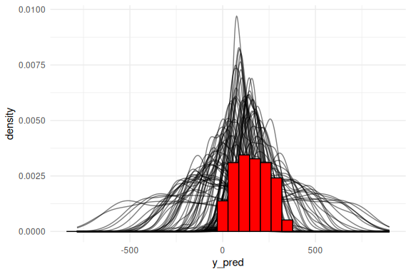 The posterior predictive checks also do not look great! Lets look at it as densities:
# same as above just with densities instead of histograms

as_draws_df(fit$draws(c("a","b","sigma"))) %>%
  select(-contains(".")) %>% mutate(draw = 1:n(),
                                    x = list(seq(0,100, length.out = N))) %>%
  filter(draw %in% draw_id) %>%
  unnest((x)) %>%
  mutate(y_pred = rnorm(n(),a+b*x,exp(sigma))) %>%
  ggplot()+
  geom_line(aes(x = y_pred, group = draw), col = "black", alpha = 0.5, stat = "density")+
  geom_density(data = data.frame(y = y),aes(x = y, after_stat(density)), col = "red")+
  theme_minimal()
## Warning: Dropping 'draws_df' class as required metadata was removed.
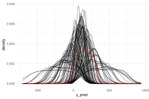
Not great! Lets plot them as conditional on the explanatory variable (x).
# same as above now we just do not get our predictions from a normal distribution,
# but instead we just plot the mean prediction "a+b*x" as a line plot.


as_draws_df(fit$draws(c("a","b","sigma"))) %>%
  select(-contains(".")) %>% mutate(draw = 1:n(),
                                    x = list(seq(0,100, length.out = N))) %>%
  unnest((x)) %>%
  filter(draw %in% draw_id) %>%
  mutate(y_pred_mu = a+b*x) %>%
  ggplot()+
  geom_line(aes(x = x, y = y_pred_mu, group = draw), col = "black", alpha = 0.05)+
  geom_point(data = data.frame(y = y,x=x),aes(x = x, y = y), col = "red")+
  theme_minimal()
## Warning: Dropping 'draws_df' class as required metadata was removed.
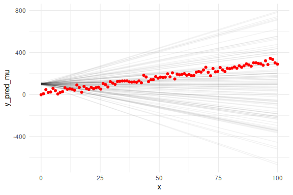
We can also overlay the 95 % prediction interval, by including sigma.
# same as above now we just do not get our predictions from a normal distribution,
# but instead we just plot the mean prediction "a+b*x" as a line plot.

as_draws_df(fit$draws(c("a","b","sigma"))) %>%
  select(-contains(".")) %>% mutate(draw = 1:n(),
                                    x = list(seq(0,100, length.out = N))) %>%
  unnest((x)) %>%
  filter(draw %in% draw_id) %>%
  # Adding two extra terms for the prediction intervals (here we use 2 instead of 1.96 for 95%)
  # Note again the exponentiation!
  mutate(y_pred_mu = a+b*x,
         y_pred_low = a+b*x - 2 * exp(sigma),
         y_pred_high = a+b*x + 2 * exp(sigma)
         ) %>%
  ggplot()+
  # the prediction ribbon:
  geom_ribbon(aes(x = x, ymin = y_pred_low, ymax = y_pred_high, group = draw), fill = "grey", alpha = 0.005)+
  geom_line(aes(x = x, y = y_pred_mu, group = draw), col = "black", alpha = 0.05)+
  geom_point(data = data.frame(y = y,x=x),aes(x = x, y = y), col = "red")+
  theme_minimal()
## Warning: Dropping 'draws_df' class as required metadata was removed.
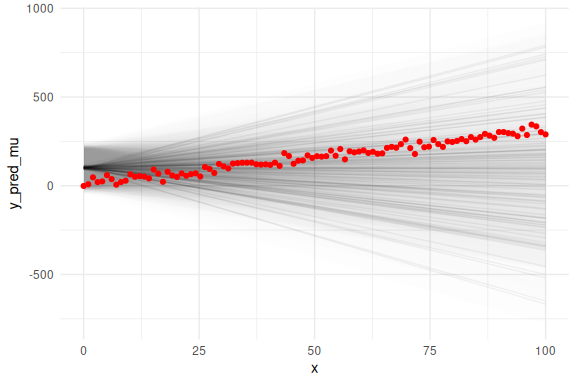
All these plots tell us that there is something wrong with the model. The posterior distribution of the parameters are not within the priors for the intercept and which means that these priors for this model are not well suited (because we forgot to add the slope in the model). Next the prior for the slope is exactly the posterior, again hitting at problems. The posterior predictive plots are even more telling showing how the model does not fit the data and the last plot with the overlaid data shows that there is something wrong with the slope of the line.
Pyschometric function
Now we move to another example of problems that might arise. Here i also want to showcase some the sampler parameters that one can tweak, both for optimal inference and convergence, but also for speed and convenience. For this next section we will be looking the the psychometric function which i introduced in the “data simulation markdown”.
A Short reminder of the psychometric model; We assume that agents get a “stimulus” value (x) that they give a binary choice (y) to. This binary choice stems from a probability that is dependent on the stimulus and three subject level parameters (threshold),
(slope) and
(lapse rate). These three parameters govern the shape of the psychometric, see the data simulation markdown if this does not make sense.
Starting by simulating a single agent
#data points
N = 100
#threshold
alpha = 20
#slope
beta = 3
#lapse
lambda = 0.05
#x's
x = seq(0,40, length.out = N)
# getting the probabilities from the model and the parameters
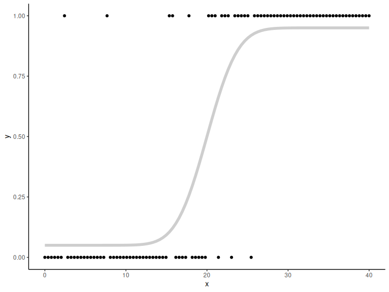
p = lambda+(1-2*lambda)*(0.5+0.5*pracma::erf((x-alpha)/(sqrt(2)*beta)))
Plotting the probabilities
data.frame() %>% ggplot(aes(x =x,y = p))+
  geom_point()+
  theme_classic()
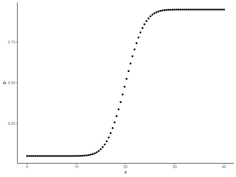
These are the latent probabilities that we wont see with experimental data. We would only see the realization of these (i.e the binary choice).
Plotting both:
# generating binary responses from the probabilities above
y = rbinom(N,1,p)

data.frame() %>% ggplot(aes(x =x,y = y))+
  geom_point()+
  theme_classic()+
  geom_line(aes(x = x, y = p), col = "grey", alpha = 0.75, linewidth = 2)
Before we write our Stan model, we now have to make sure that we understand our model, and its parameters. From the data simulation markdown we saw that could be any value from ]-
to
[ as it just moves the location of the function.
on the other hand had to be positive as its the standard deviation of the underlying normal distribution. Lastly
is the lapse rate and governed what probability (y) the functions asymtotes to at x approaches -
but also when x approaches
but the value just being 1-
. This would mean that if we want to keep the shape of the function (y increases as x increases) lambda must be below 0.5, as values above 0.5 would make the function decrease as x increases (i.e. flip the function around the threshold).
If this is not clear go back to the data simulation markdown and simulate different values of these parameters and see how the function changes shape.
constrains
To ensure that stan knows about our constraints we are going to use transformations as in the prior markdown. Here we will use the exponential for to keep it positive. For
we are going to use the inverse_logit transformation, which transforms a value from ]-
;
[ to ]0 ; 1[. We further then need to divide it by 2 to get it inside the ]0 ; 0.5[ constraint.
Now we can write our Stan model and fit the stimulus (x) and the binary responses (y) to get estimates of the simulated parameters.
//This block defines the input that. So these things needs to go into the model
data {
  //Define the number of datapoints this is defined by an integer
  int N;
  //Define an array called y that is as long as the number of datapoints (i.e. N) (Note these are integers)
  array[N] int y;
  // same as y but a variable called x our independent variable
  vector[N] x;
}

// This is the parameters block. Here we define the free parameters
// which are the onces that STAN estimates for us.
// this is again a,b and sigma
parameters {
  real alpha;
  real beta;
  real lambda;
}

// This is the model block here we define our model.

model {
  y ~ bernoulli(inv_logit(lambda)/2+(1-2*inv_logit(lambda)/2)*(0.5+0.5*erf((x-alpha)/(sqrt(2)*exp(beta)))));
}
Now we fit the model to the data by entering our data.
As an additional step we will here specify that we only want half the warm-up and samples and only 3 parallel chains. The reason to do this is two-fold, the model without priors as specified above will not sample properly and will thus take around 5-10 seconds per chain (so we save some time). The other reason is to showcase this feature.
# Fit the STAN model
fit = model_obj2$sample(data = list(N =N, x = x, y =y),
                        seed = seeds,
                        #warm-up samples
                        iter_warmup = 500,
                        #inference samples
                        iter_sampling = 500,
                        #chains
                        chains = 3,
                        #parallel chains
                        parallel_chains = 3)
## Running MCMC with 3 parallel chains...
##
## Chain 1 Iteration:   1 / 1000 [  0%]  (Warmup)
## Chain 2 Iteration:   1 / 1000 [  0%]  (Warmup)
## Chain 2 Iteration: 100 / 1000 [ 10%]  (Warmup)
## Chain 3 Iteration:   1 / 1000 [  0%]  (Warmup)
## Chain 1 Iteration: 100 / 1000 [ 10%]  (Warmup)
## Chain 2 Iteration: 200 / 1000 [ 20%]  (Warmup)
## Chain 2 Iteration: 300 / 1000 [ 30%]  (Warmup)
## Chain 2 Iteration: 400 / 1000 [ 40%]  (Warmup)
## Chain 2 Iteration: 500 / 1000 [ 50%]  (Warmup)
## Chain 2 Iteration: 501 / 1000 [ 50%]  (Sampling)
## Chain 2 Iteration: 600 / 1000 [ 60%]  (Sampling)
## Chain 2 Iteration: 700 / 1000 [ 70%]  (Sampling)
## Chain 1 Iteration: 200 / 1000 [ 20%]  (Warmup)
## Chain 2 Iteration: 800 / 1000 [ 80%]  (Sampling)
## Chain 2 Iteration: 900 / 1000 [ 90%]  (Sampling)
## Chain 2 Iteration: 1000 / 1000 [100%]  (Sampling)
## Chain 2 finished in 0.5 seconds.
## Chain 1 Iteration: 300 / 1000 [ 30%]  (Warmup)
## Chain 3 Iteration: 100 / 1000 [ 10%]  (Warmup)
## Chain 1 Iteration: 400 / 1000 [ 40%]  (Warmup)
## Chain 1 Iteration: 500 / 1000 [ 50%]  (Warmup)
## Chain 1 Iteration: 501 / 1000 [ 50%]  (Sampling)
## Chain 3 Iteration: 200 / 1000 [ 20%]  (Warmup)
## Chain 1 Iteration: 600 / 1000 [ 60%]  (Sampling)
## Chain 1 Iteration: 700 / 1000 [ 70%]  (Sampling)
## Chain 3 Iteration: 300 / 1000 [ 30%]  (Warmup)
## Chain 1 Iteration: 800 / 1000 [ 80%]  (Sampling)
## Chain 1 Iteration: 900 / 1000 [ 90%]  (Sampling)
## Chain 3 Iteration: 400 / 1000 [ 40%]  (Warmup)
## Chain 1 Iteration: 1000 / 1000 [100%]  (Sampling)
## Chain 1 finished in 3.1 seconds.
## Chain 3 Iteration: 500 / 1000 [ 50%]  (Warmup)
## Chain 3 Iteration: 501 / 1000 [ 50%]  (Sampling)
## Chain 3 Iteration: 600 / 1000 [ 60%]  (Sampling)
## Chain 3 Iteration: 700 / 1000 [ 70%]  (Sampling)
## Chain 3 Iteration: 800 / 1000 [ 80%]  (Sampling)
## Chain 3 Iteration: 900 / 1000 [ 90%]  (Sampling)
## Chain 3 Iteration: 1000 / 1000 [100%]  (Sampling)
## Chain 3 finished in 7.1 seconds.
##
## All 3 chains finished successfully.
## Mean chain execution time: 3.6 seconds.
## Total execution time: 7.2 seconds.

## Warning: 496 of 1500 (33.0%) transitions ended with a divergence.
## See https://mc-stan.org/misc/warnings for details.

## Warning: 564 of 1500 (38.0%) transitions hit the maximum treedepth limit of 10.
## See https://mc-stan.org/misc/warnings for details.
That took a dangerous long time and there are a lot of warnings from the Stan output. Something must have gone wrong. Checking the output:
fit
##  variable          mean median           sd          mad            q5
##    lp__   -4.324000e+01 -31.18 1.851000e+01 3.950000e+00 -6.931000e+01
##    alpha  -1.178591e+08  19.40 2.444369e+08 2.980000e+00 -6.810056e+08
##    beta    1.068000e+01   1.70 2.294300e+02 6.390000e+00 -4.344800e+02
##    lambda -4.562523e+13  -1.98 7.778555e+13 7.430902e+09 -2.189512e+14
##            q95 rhat ess_bulk ess_tail
##         -27.86 2.26        3        3
##    33508800.00 2.00        5       11
##         511.13 1.90       28       57
##  6050627500.00 3.18        3       15
Looking at the summary statistics of the model we see that the parameters are all over the place very big/small. The sampler diagnoistics for the parameters are also terrible with high rhat and very low ess_bulk and ess_tail. Lets look at the trace plots
mcmc_trace(fit$draws(c("alpha","beta","lambda")))
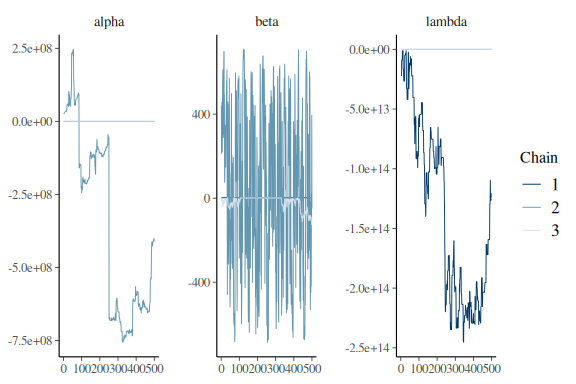
That is not hairy caterpillars.
One could go on and plot prior-posterior updates and predictive checks, but the experienced modeller would here already know the problem; we did not specify any priors on the model. One should now go back to the prior markdown and investigate what kind of distribution of values are sensible for their design and then select prior values based on that. Here we move on with priors that would work in this psychophysical experiment (also based on what we used for the simulation).
//This block defines the input that. So these things needs to go into the model
data {
  //Define the number of datapoints this is defined by an integer
  int N;
  //Define an array called y that is as long as the number of datapoints (i.e. N) (Note these are integers)
  array[N] int y;
  // same as y but a variable called x our independent variable
  vector[N] x;
}

// This is the parameters block.
// Here we define the free parameters which are the onces that STAN estimates for us.
// this is again a,b and sigma
parameters {
  real alpha;
  real beta;
  real lambda;
}

// This is the model block here we define the model.

model {
  //priors for the model
  alpha ~ normal(0,20);
  beta ~ normal(0,3);
  lambda ~ normal(-4,2);

  y ~ bernoulli(inv_logit(lambda)/2+(1-2*inv_logit(lambda)/2)*(0.5+0.5*erf((x-alpha)/(sqrt(2)*exp(beta)))));
}
Now collect 4 parallel chains (this is what is usually done). Now we also specify that stan should only print the sampling statements after each 250 iterations
# Fit the STAN model
fit = model_obj2$sample(data = list(N =N, x = x, y =y),
                        seed = seeds,
                        #warm-up samples
                        iter_warmup = 500,
                        #inference samples
                        iter_sampling = 500,
                        #chains
                        chains = 4,
                        #parallel chains
                        parallel_chains = 4,
                        #refresh rate of printing
                        refresh = 250)
## Running MCMC with 4 parallel chains...
##
## Chain 1 Iteration:   1 / 1000 [  0%]  (Warmup)
## Chain 1 Iteration: 250 / 1000 [ 25%]  (Warmup)
## Chain 1 Iteration: 500 / 1000 [ 50%]  (Warmup)
## Chain 1 Iteration: 501 / 1000 [ 50%]  (Sampling)
## Chain 1 Iteration: 750 / 1000 [ 75%]  (Sampling)
## Chain 1 Iteration: 1000 / 1000 [100%]  (Sampling)
## Chain 2 Iteration:   1 / 1000 [  0%]  (Warmup)
## Chain 2 Iteration: 250 / 1000 [ 25%]  (Warmup)
## Chain 2 Iteration: 500 / 1000 [ 50%]  (Warmup)
## Chain 2 Iteration: 501 / 1000 [ 50%]  (Sampling)
## Chain 2 Iteration: 750 / 1000 [ 75%]  (Sampling)
## Chain 2 Iteration: 1000 / 1000 [100%]  (Sampling)
## Chain 3 Iteration:   1 / 1000 [  0%]  (Warmup)
## Chain 3 Iteration: 250 / 1000 [ 25%]  (Warmup)
## Chain 3 Iteration: 500 / 1000 [ 50%]  (Warmup)
## Chain 3 Iteration: 501 / 1000 [ 50%]  (Sampling)
## Chain 3 Iteration: 750 / 1000 [ 75%]  (Sampling)
## Chain 3 Iteration: 1000 / 1000 [100%]  (Sampling)
## Chain 4 Iteration:   1 / 1000 [  0%]  (Warmup)
## Chain 4 Iteration: 250 / 1000 [ 25%]  (Warmup)
## Chain 4 Iteration: 500 / 1000 [ 50%]  (Warmup)
## Chain 4 Iteration: 501 / 1000 [ 50%]  (Sampling)
## Chain 4 Iteration: 750 / 1000 [ 75%]  (Sampling)
## Chain 4 Iteration: 1000 / 1000 [100%]  (Sampling)
## Chain 1 finished in 0.1 seconds.
## Chain 2 finished in 0.1 seconds.
## Chain 3 finished in 0.1 seconds.
## Chain 4 finished in 0.1 seconds.
##
## All 4 chains finished successfully.
## Mean chain execution time: 0.1 seconds.
## Total execution time: 0.3 seconds.
Much faster, but wait we still see a small amount of divergences!
Lets check the summary and the traceplots!
fit
##  variable   mean median   sd  mad     q5    q95 rhat ess_bulk ess_tail
##    lp__   -29.54 -29.31 1.27 1.22 -31.90 -28.02 1.01      599     1078
##    alpha   19.73  19.78 1.08 1.03  17.87  21.51 1.01      886      775
##    beta     1.17   1.37 0.88 0.38  -0.74   1.96 1.01      354      190
##    lambda  -3.12  -2.96 1.18 0.98  -5.27  -1.61 1.01      478      584
Looking at the summary statistics of the model we see that the parameter diagnoistics are much better, and also the mean and standard deviation. However the slope (beta) and partly the lapse (lambda) parameter is still not sufficiently good.
Lets look at the traceplot
mcmc_trace(fit$draws(c("alpha","beta","lambda")))
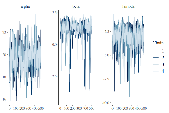
These look much better than before, but we still need to remove the last couple of divergences. and make the chains look better especially for the slope (beta) parameter.
We could do this by making our priors more informative especially the slope as our prior on this is very wide (as its exponentiated).
However another option is to make the sampler work a bit harder which can be done with the “adapt_delta” argument. This argument takes a value between 0 and 1 (not including these) and basically tells the sampler how hard it has to work, higher values means longer sample time but the chance of divergences are also smaller.
Normally we only want to increase this with quite few divergences, i.e. it wouldn’t have helped above without priors. The default adapt_delta is 0.9. Lets set it to 0.99 and see the results.
# Fit the STAN model
fit = model_obj2$sample(data = list(N =N, x = x, y =y),
                        seed = seeds,
                        #warm-up samples
                        iter_warmup = 500,
                        #inference samples
                        iter_sampling = 500,
                        #chains
                        chains = 4,
                        #parallel chains
                        parallel_chains = 4,
                        #refresh rate of printing
                        refresh = 250,
                        #adap delta argument
                        adapt_delta = 0.99)
## Running MCMC with 4 parallel chains...
##
## Chain 1 Iteration:   1 / 1000 [  0%]  (Warmup)
## Chain 1 Iteration: 250 / 1000 [ 25%]  (Warmup)
## Chain 2 Iteration:   1 / 1000 [  0%]  (Warmup)
## Chain 2 Iteration: 250 / 1000 [ 25%]  (Warmup)
## Chain 3 Iteration:   1 / 1000 [  0%]  (Warmup)
## Chain 4 Iteration:   1 / 1000 [  0%]  (Warmup)
## Chain 4 Iteration: 250 / 1000 [ 25%]  (Warmup)
## Chain 4 Iteration: 500 / 1000 [ 50%]  (Warmup)
## Chain 4 Iteration: 501 / 1000 [ 50%]  (Sampling)
## Chain 1 Iteration: 500 / 1000 [ 50%]  (Warmup)
## Chain 1 Iteration: 501 / 1000 [ 50%]  (Sampling)
## Chain 2 Iteration: 500 / 1000 [ 50%]  (Warmup)
## Chain 2 Iteration: 501 / 1000 [ 50%]  (Sampling)
## Chain 4 Iteration: 750 / 1000 [ 75%]  (Sampling)
## Chain 4 Iteration: 1000 / 1000 [100%]  (Sampling)
## Chain 4 finished in 0.2 seconds.
## Chain 1 Iteration: 750 / 1000 [ 75%]  (Sampling)
## Chain 1 Iteration: 1000 / 1000 [100%]  (Sampling)
## Chain 2 Iteration: 750 / 1000 [ 75%]  (Sampling)
## Chain 1 finished in 0.3 seconds.
## Chain 2 Iteration: 1000 / 1000 [100%]  (Sampling)
## Chain 2 finished in 0.5 seconds.
## Chain 3 Iteration: 250 / 1000 [ 25%]  (Warmup)
## Chain 3 Iteration: 500 / 1000 [ 50%]  (Warmup)
## Chain 3 Iteration: 501 / 1000 [ 50%]  (Sampling)
## Chain 3 Iteration: 750 / 1000 [ 75%]  (Sampling)
## Chain 3 Iteration: 1000 / 1000 [100%]  (Sampling)
## Chain 3 finished in 0.7 seconds.
##
## All 4 chains finished successfully.
## Mean chain execution time: 0.4 seconds.
## Total execution time: 0.9 seconds.
Took quite a bit longer but no divergences. Lets check the summary statistics and traceplots again.
fit
##  variable   mean median   sd  mad     q5    q95 rhat ess_bulk ess_tail
##    lp__   -29.51 -29.29 1.20 1.17 -31.76 -28.05 1.01      385      965
##    alpha   19.74  19.80 1.06 1.07  17.98  21.42 1.01      600      955
##    beta     1.21   1.38 0.83 0.39  -0.21   1.96 1.01      415      208
##    lambda  -3.10  -2.96 1.09 0.95  -5.14  -1.69 1.01      415      400
Looking at the summary statistics of the model we see that the parameters are much better. Lets look at the traceplots.
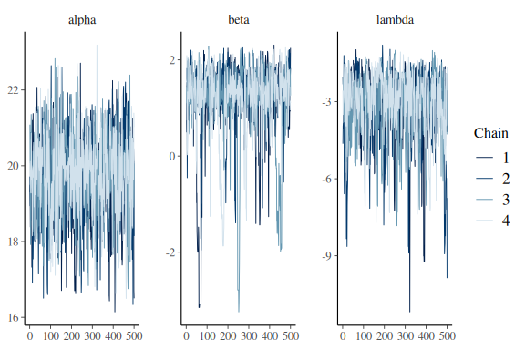
mcmc_trace(fit$draws(c("alpha","beta","lambda")))
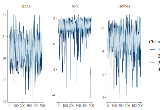 This isn’t to great especially for the slope beta.
Lets demonstrate the other option of changing the priors slightly:
//This block defines the input that. So these things needs to go into the model
data {
  //Define the number of datapoints this is defined by an integer
  int N;
  //Define an array called y that is as long as the number of datapoints (i.e. N) (Note these are integers)
  array[N] int y;
  // same as y but a variable called x our independent variable
  vector[N] x;
}

// This is the parameters block. Here we define the free parameters which are the onces that STAN estimates for us.
// this is again a,b and sigma
parameters {
  real alpha;
  real beta;
  real lambda;
}

// This is the model block here we define how we believe the model is (of cause we simulated the data so we just put in the same thing as we did when simulating)

model {
  //priors for the model
  alpha ~ normal(10,20);
  beta ~ normal(0,2);
  lambda ~ normal(-4,2);

  y ~ bernoulli(inv_logit(lambda)/2+(1-2*inv_logit(lambda)/2)*(0.5+0.5*erf((x-alpha)/(sqrt(2)*exp(beta)))));
}
Fitting the model
# Fit the STAN model
fit = model_obj2$sample(data = list(N =N, x = x, y =y),
                        seed = seeds,
                        #warm-up samples
                        iter_warmup = 500,
                        #inference samples
                        iter_sampling = 500,
                        #chains
                        chains = 4,
                        #parallel chains
                        parallel_chains = 4,
                        #refresh rate of printing
                        refresh = 250,
                        #adap delta argument default 0.9
                        adapt_delta = 0.9)
## Running MCMC with 4 parallel chains...
##
## Chain 1 Iteration:   1 / 1000 [  0%]  (Warmup)
## Chain 1 Iteration: 250 / 1000 [ 25%]  (Warmup)
## Chain 1 Iteration: 500 / 1000 [ 50%]  (Warmup)
## Chain 1 Iteration: 501 / 1000 [ 50%]  (Sampling)
## Chain 1 Iteration: 750 / 1000 [ 75%]  (Sampling)
## Chain 1 Iteration: 1000 / 1000 [100%]  (Sampling)
## Chain 2 Iteration:   1 / 1000 [  0%]  (Warmup)
## Chain 2 Iteration: 250 / 1000 [ 25%]  (Warmup)
## Chain 2 Iteration: 500 / 1000 [ 50%]  (Warmup)
## Chain 2 Iteration: 501 / 1000 [ 50%]  (Sampling)
## Chain 2 Iteration: 750 / 1000 [ 75%]  (Sampling)
## Chain 2 Iteration: 1000 / 1000 [100%]  (Sampling)
## Chain 3 Iteration:   1 / 1000 [  0%]  (Warmup)
## Chain 3 Iteration: 250 / 1000 [ 25%]  (Warmup)
## Chain 3 Iteration: 500 / 1000 [ 50%]  (Warmup)
## Chain 3 Iteration: 501 / 1000 [ 50%]  (Sampling)
## Chain 3 Iteration: 750 / 1000 [ 75%]  (Sampling)
## Chain 3 Iteration: 1000 / 1000 [100%]  (Sampling)
## Chain 4 Iteration:   1 / 1000 [  0%]  (Warmup)
## Chain 4 Iteration: 250 / 1000 [ 25%]  (Warmup)
## Chain 4 Iteration: 500 / 1000 [ 50%]  (Warmup)
## Chain 4 Iteration: 501 / 1000 [ 50%]  (Sampling)
## Chain 4 Iteration: 750 / 1000 [ 75%]  (Sampling)
## Chain 4 Iteration: 1000 / 1000 [100%]  (Sampling)
## Chain 1 finished in 0.1 seconds.
## Chain 2 finished in 0.1 seconds.
## Chain 3 finished in 0.1 seconds.
## Chain 4 finished in 0.1 seconds.
##
## All 4 chains finished successfully.
## Mean chain execution time: 0.1 seconds.
## Total execution time: 0.4 seconds.
Summary and traceplots
fit
##  variable   mean median   sd  mad     q5    q95 rhat ess_bulk ess_tail
##    lp__   -29.45 -29.24 1.33 1.31 -32.02 -27.81 1.00      576      874
##    alpha   19.70  19.81 1.12 1.10  17.75  21.42 1.00      921      957
##    beta     1.17   1.36 0.82 0.41  -0.69   1.97 1.01      286      144
##    lambda  -3.19  -2.93 1.32 1.07  -5.76  -1.57 1.00      398      405
mcmc_trace(fit$draws(c("alpha","beta","lambda")))
 No divergences, no tree_depth, and better traceplots.
Final remarks
This finishes the section on diagnostics, at least for now. One thing that I haven’t touched on which i mentioned in the beginning is parameterization. This terms refers to the fact that some models can be written (in stan code) in many different ways that either make it easier or harder for the sampler to explore the joint posterior distribution. We will come back to this in one of the next markdowns the “hierarchical models markdown”. Here we will explore parameterization and the diagnoistics we encounter there and how to fix it.
The main takeaway from this markdown should be that diagnosing issues with the stan model is more of an art and not a science. Experience is one of the best bets for being able to find the problems of a model quickly, but sometimes this fails.