
Hierarchical Models
Published:
- Bayesian Workflow
This R markdown is an introduction to fitting Hierarchical models in stan.
Table of content
Overview
Hierarchical models is probably the term with the most diverse number of names in the litterature; Mixed / random effects, multilevel and hierarchical models just to name a few.
In the simplest term these types of model allows one to model data that has inherent structure. Here we will mainly focus on having several subjects completing the same experiment.
This essentially means we want to build a model that can account for the fact that we have different individuals completing the same task. So instead of having to model these individuals separately we build a model that models all the individuals together. We do this by assuming they are from a similar underlying distribution (population?).
These types of models thus allows to estimate individual level parameters for each subject, but also group level statistics, which is something you do not get for free without hierarchical models. These group level statistics are what is usually of interest in many tasks as we want to see differences between groups based on some experimentally manipulated variable.
The concept of hierarchical models are quite simple and are best illustrated by a figure stolen from here
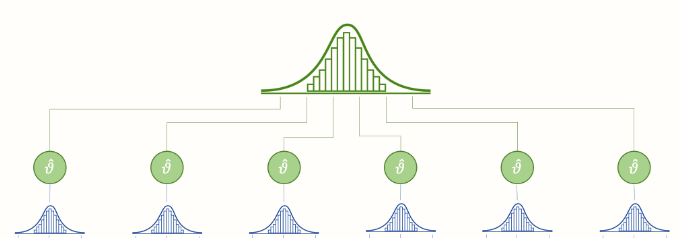
Here the uppermost distribution represents the group level distribution for a parameter, and the individual smaller distributions below are the subject level distributions of the parameter.
What we will normally assume is that our group level parameters are normally distributed and then we draw subject level parameters from this group level distribution.
Before demonstrating this through our Bayesian workflow, where we write our models in stan we might start with the more familiar lmer syntax. Here we’ll look at a hierarchical linear (mixed) effects model with the following lmer syntax: y ~ x + (x | id). Which spelled out means we model y as a function of x for where each subject get their own slope and intercept (e.g. (x | id) syntax).
We will also look at the uncertainty of this linear model i.e. sigma later, but for now we keep it fixed for all subjects as this is what is assumed by the usual lmer model.
Simulations:
We start with simulating some parameter values for our agents and then plot them:
#number of simulated subjects
n_sub = 20
#number of simulated trials
n_trials = 100

#intercepts:
int = rnorm(n_sub,0,50)
#slopes:
slopes = rnorm(n_sub,3,3)
#sigma
sigma = 50

#x values
xs = seq(0,50,length.out = n_trials)

# simulate trialwise responses:
df = data.frame(intercept = int, slopes = slopes,sigma = sigma) %>%
  mutate(id = 1:n_sub,
         x = list(seq(0,50,length.out = n_trials))) %>%
  unnest(x) %>% rowwise() %>%
  mutate(y_mean = intercept + x * slopes,
         y_pred = rnorm(1,intercept + x * slopes, sigma))
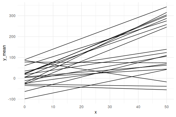
plotting these without sigma (e.g. one line per subject):
df %>%
  ggplot(aes(x = x, y = y_mean,group = id))+
  geom_line()+
  theme_minimal()
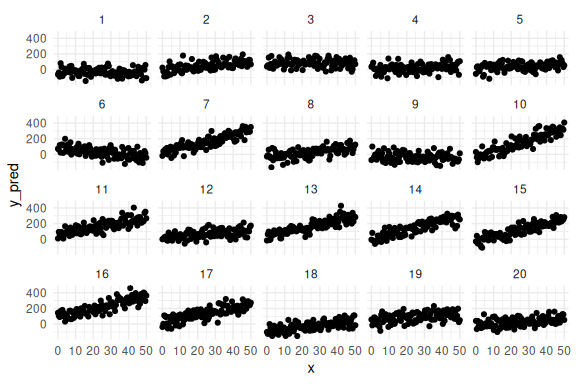
Individual data points for each subject.
df %>%
  ggplot(aes(x = x, y = y_pred,group = id))+
  geom_point()+
  facet_wrap(~id)+
  theme_minimal()
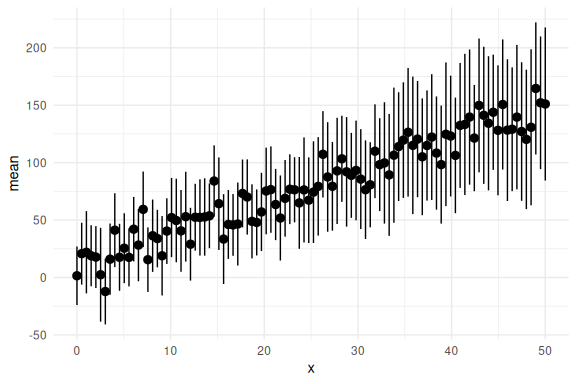
and lastly the group level (aggregating over subjects):
df %>%
  group_by(x) %>%
  summarize(mean = mean(y_pred), se = sd(y_pred)/sqrt(n())) %>%
  ggplot(aes(x = x, y = mean))+
  geom_pointrange(aes(ymin = mean-2*se,ymax = mean+2*se))+
  theme_minimal()
Please note that one could fit these subjects individually and then combine their parameters estimates to gain a group level estimate. In code this would amount to looping through each subject with an individual level model and then collecting their parameter estimates. Inorder to then acheive a group level estimate for the parameters one would use error-proporgation, for instance bootstrapping to get a group level mean and standard deviation of each parameter estimate.
We here start by showing this apporach to compare it to the full hierarchical model. Taking the stancode from the model fitting markdown we have:
Note, here we also add some vague priors to help the sampler:
//This block defines the input that. So these things needs to go into the model
data {
  //Define the number of datapoints this is defined by an integer
  int N;
  //Define a vector called y that is as long as the number of datapoints (i.e. N)
  vector[N] y;
  // same as y but a variable called x our independent variable
  vector[N] x;
}

// This is the parameters block.
// Here we define the free parameters which are the onces that STAN estimates for us.
// this is again a,b and sigma
parameters {
  real a;
  real b;
  real sigma;
}

// This is the model block here we define the model.

model {
  //priors
  a ~ normal(0,500);
  b ~ normal(0,10);
  sigma ~ normal(0,5);

  y ~ normal(a+b*x, exp(sigma));
}
Now we loop though each of our subjects and collect the summary of their parameters:
#initalize an empty dataframe to collect all the information
parameters = data.frame()
for(sub in unique(df$id)){

  #subset the data
  df1 = df %>% filter(id == sub)

  # fit the model to the subsetted data
  fit = model_obj2$sample(data = list(N = nrow(df1), x = df1$x, y = df1$y_pred),
                          seed = seeds,
                          refresh = 0)

  # collect parameters
  param_sum = fit$summary(c("a","b","sigma"))

  # collect diagnoistics
  diag= data.frame(fit$diagnostic_summary())

  #collect all the information in one dataframe
  param_sum = param_sum %>%
    mutate(id = sub,
           div = mean(diag$num_divergent),
           tree = mean(diag$num_max_treedepth),
           energy = mean(diag$ebfmi),
  )

  #combine it all
  parameters = rbind(parameters,param_sum)
}
## Running MCMC with 4 sequential chains...
##
## Chain 1 finished in 0.1 seconds.
## Chain 2 finished in 0.1 seconds.
## Chain 3 finished in 0.1 seconds.
## Chain 4 finished in 0.1 seconds.
##
## All 4 chains finished successfully.
## Mean chain execution time: 0.1 seconds.
## Total execution time: 0.7 seconds.
##
## Running MCMC with 4 sequential chains...
##
## Chain 1 finished in 0.1 seconds.
## Chain 2 finished in 0.1 seconds.
## Chain 3 finished in 0.1 seconds.
## Chain 4 finished in 0.1 seconds.
##
## All 4 chains finished successfully.
## Mean chain execution time: 0.1 seconds.
## Total execution time: 0.6 seconds.
##
## Running MCMC with 4 sequential chains...
##
## Chain 1 finished in 0.1 seconds.
## Chain 2 finished in 0.1 seconds.
## Chain 3 finished in 0.1 seconds.
## Chain 4 finished in 0.1 seconds.
##
## All 4 chains finished successfully.
## Mean chain execution time: 0.1 seconds.
## Total execution time: 0.6 seconds.
Checking model diagnoistics
parameters %>% select(rhat,ess_bulk,ess_tail,div,tree,energy) %>%
  pivot_longer(everything()) %>%
  ggplot(aes(x = value))+geom_histogram(col = "black")+
  facet_wrap(~name, scales = "free")
## `stat_bin()` using `bins = 30`. Pick better value with `binwidth`.
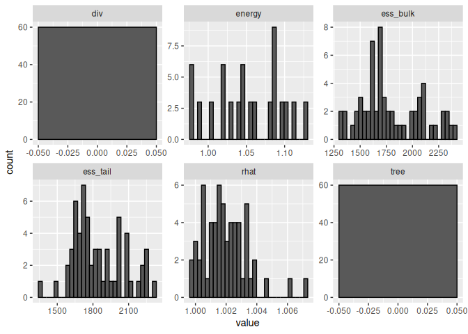
No divergences, no tree depth, Rhat values close to 1 and effective sample sizes (ess_*) very high; looks good!
Now we can look how well each fit, fits the individual data points here firstly just the mean predictions and their 95% credibility interval:
# wrangle the parameters dataframe to get the mean and 95% Credibility interval:

params = parameters %>% select(mean,q5,q95,variable,id) %>%
  pivot_wider(values_from = c("mean","q5","q95"), names_from = variable) %>%
  mutate(x = list(seq(0,50,length.out = n_trials))) %>%
  unnest(x) %>% rowwise() %>%
  mutate(y_mean = mean_a + mean_b * x,
         y_q5 = q5_a + q5_b * x,
         y_q95 = q95_a + q95_b * x)


df %>%
  ggplot(aes(x = x, y = y_pred,group = id))+
  geom_point()+
  geom_line(data = params, aes(x = x, y = y_mean), col = "red")+
  geom_ribbon(data = params, aes(x = x, y = y_mean, ymin = y_q5, ymax = y_q95), fill = "red", alpha = 0.75)+
  facet_wrap(~id)+
  theme_minimal()
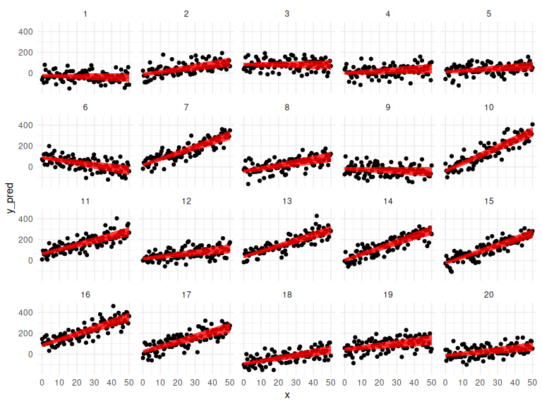
This looks really good! Now we can also check the group level if we propagate the uncertainty from each individual. This is essentially wrong as we assume that all the parameters follow a normal distribution which is not necessarily the case!
params = parameters %>%
  select(mean,sd,variable,id) %>%
  mutate(replicate = list(1:100)) %>%
  unnest() %>%
  rowwise() %>%
  mutate(draw = rnorm(n(),mean,sd)) %>%
  group_by(replicate,variable) %>%
  summarize(draw = mean(draw)) %>%
  select(draw,variable,replicate) %>%
  pivot_wider(names_from = "variable",values_from = "draw") %>%
  unnest() %>%
  mutate(x = list(seq(0,50,length.out = n_trials))) %>%
  unnest(x) %>%
  rowwise() %>%
  mutate(y_mean = a + b * x,
         y_low = a + b * x - 2 * exp(sigma),
         y_high = a + b * x + 2 * exp(sigma))
## Warning: `cols` is now required when using `unnest()`.
## ℹ Please use `cols = c(replicate)`.

## `summarise()` has grouped output by 'replicate'. You can override using the
## `.groups` argument.

## Warning: `cols` is now required when using `unnest()`.
## ℹ Please use `cols = c()`.
df %>% group_by(x) %>%
  summarize(mean = mean(y_pred), se = sd(y_pred)/sqrt(n())) %>%
  ggplot(aes(x = x, y = mean))+
  geom_pointrange(aes(ymin = mean-2*se,ymax = mean+2*se))+
    geom_line(data = params, aes(x = x, y = y_mean, group = replicate), col = "red", alpha = 0.1)+
  theme_minimal()
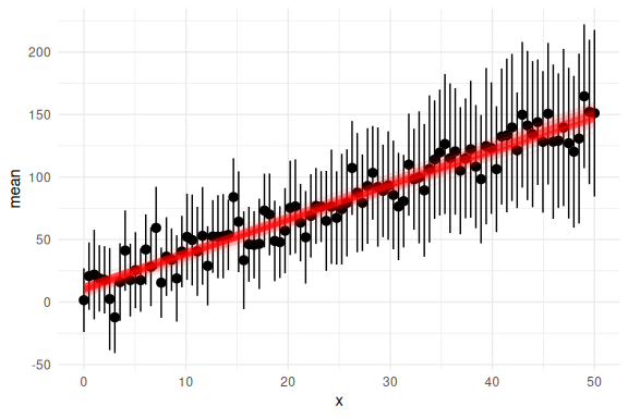
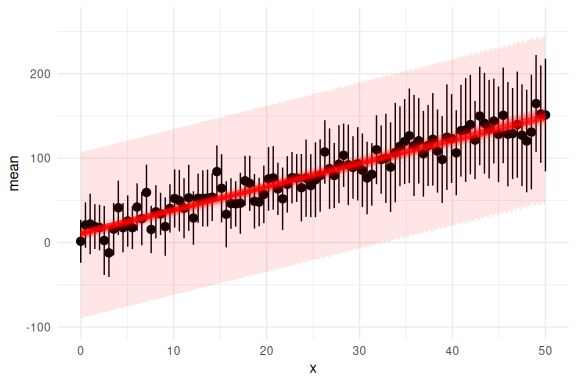
And with the prediction intervals:
df %>% group_by(x) %>%
  summarize(mean = mean(y_pred), se = sd(y_pred)/sqrt(n())) %>%
  ggplot(aes(x = x, y = mean))+
  geom_pointrange(aes(ymin = mean-2*se,ymax = mean+2*se))+
    geom_line(data = params, aes(x = x, y = y_mean, group = replicate), col = "red", alpha = 0.1)+
  geom_ribbon(data = params, aes(x = x, y = y_mean, ymin = y_low, ymax = y_high),
              fill = "red", alpha = 0.1)+
  theme_minimal()
Hierarchical Implementation
Now we build the Hierarchical model.
The main idea is that each of our free parameters for each subject is drawn from the same group level distribution (first plot in this markdown). In the case where we assume a normal distribution for the group level we would have:
This would thus entail that we just set priors on the group level parameters and let the model do the rest: Before we code it up we need to consider what goes into the model!
Firstly we need to provide stan with 2 additional arguments. The number of subjects, but also a identifier for which subject this trial belongs to.
//This block defines the input that. So these things needs to go into the model
data {

  //Define the number of datapoints this is defined by an integer
  int N;

  //Define the number of subjects this is defined by an integer
  int S;

  //identifier for which subject this trial belongs to
  array[N] int  S_id;

  //Define a vector called y that is as long as the number of datapoints (i.e. N)
  vector[N] y;
  // same as y but a variable called x our independent variable
  vector[N] x;
}

// This is the parameters block.
// Here we define the free parameters which are the onces that STAN estimates for us.
// this is again a,b and sigma
parameters {
  real mu_a;
  real sigma_a;

  vector[S] a;

  real mu_b;
  real sigma_b;

  vector[S] b;

  real mu_sigma;
  real sigma_sigma;

  vector[S] sigma;

}

// This is the model block here we define the model.

model {
  //priors
  mu_a ~ normal(0,10);
  sigma_a ~ normal(0,5);

  a ~ normal(mu_a,exp(sigma_a));

  mu_b ~ normal(0,10);
  sigma_b ~ normal(0,5);

  b ~ normal(mu_b,exp(sigma_b));

  mu_sigma ~ normal(0,3);
  sigma_sigma ~ normal(0,3);

  sigma ~ normal(mu_sigma,exp(sigma_sigma));

  for(n in 1:N){

    y[n] ~ normal(a[S_id[n]]+b[S_id[n]]*x[n], exp(sigma[S_id[n]]));

  }
}
There was alot of new stuff in this stan model. Lets go over it.
We defined two extra data arguments, the number of subjects S and an identifier for each subject belongs to what trial S_id.
We defined group and subject level parameters for each of the 3 parameters of the model. The group level parameters are called mu_* and sigma_* and are the group level parameters. We also defined a subject level parameter for each subject with the “vector[S] …(parameter)” code.
The subject level parameters are being sampled from a normal distribution with the group level means and standard deviations i.e. a ~ normal(mu_a,exp(sigma_a)).
Lastly, the particular model is defined in the trial level loop where we loop through all the trials (trials for all subjects). In this loop we use the identifier for each subject i.e. [S_id[n]] to assign each of the parameters in the vector to the right subject.
# fit the model to the subsetted data
fit = model_obj2$sample(data = list(N = nrow(df),
                                    x = df$x,
                                    y = df$y_pred,
                                    S = length(unique(df$id)),
                                    S_id = df$id),
                        seed = seeds,
                        refresh = 500,
                        iter_warmup = 500,
                        iter_sampling = 500,
                        parallel_chains = 4)
## Running MCMC with 4 parallel chains...
##
## Chain 1 Iteration:   1 / 1000 [  0%]  (Warmup)

## Chain 1 Informational Message: The current Metropolis proposal is about to be rejected because of the following issue:

## Chain 1 Exception: normal_lpdf: Scale parameter is 0, but must be positive! (in '/tmp/Rtmpn9EJTE/model-742d20b187b8.stan', line 46, column 2 to column 32)

## Chain 1 If this warning occurs sporadically, such as for highly constrained variable types like covariance matrices, then the sampler is fine,

## Chain 1 but if this warning occurs often then your model may be either severely ill-conditioned or misspecified.

## Chain 1

## Chain 2 Iteration:   1 / 1000 [  0%]  (Warmup)
## Chain 3 Iteration:   1 / 1000 [  0%]  (Warmup)
## Chain 4 Iteration:   1 / 1000 [  0%]  (Warmup)
## Chain 3 Iteration: 500 / 1000 [ 50%]  (Warmup)
## Chain 3 Iteration: 501 / 1000 [ 50%]  (Sampling)
## Chain 4 Iteration: 500 / 1000 [ 50%]  (Warmup)
## Chain 4 Iteration: 501 / 1000 [ 50%]  (Sampling)
## Chain 2 Iteration: 500 / 1000 [ 50%]  (Warmup)
## Chain 2 Iteration: 501 / 1000 [ 50%]  (Sampling)
## Chain 3 Iteration: 1000 / 1000 [100%]  (Sampling)
## Chain 3 finished in 19.7 seconds.
## Chain 4 Iteration: 1000 / 1000 [100%]  (Sampling)
## Chain 4 finished in 19.9 seconds.
## Chain 1 Iteration: 500 / 1000 [ 50%]  (Warmup)
## Chain 1 Iteration: 501 / 1000 [ 50%]  (Sampling)
## Chain 1 Iteration: 1000 / 1000 [100%]  (Sampling)
## Chain 1 finished in 22.6 seconds.
## Chain 2 Iteration: 1000 / 1000 [100%]  (Sampling)
## Chain 2 finished in 23.8 seconds.
##
## All 4 chains finished successfully.
## Mean chain execution time: 21.5 seconds.
## Total execution time: 23.9 seconds.

## Warning: 84 of 2000 (4.0%) transitions ended with a divergence.
## See https://mc-stan.org/misc/warnings for details.
Oh that looks quite bad, quite some divergences.
lets look at the summary and the trace plots for the group level parameters:
fit$summary(c("mu_a","sigma_a",
                       "mu_b","sigma_b",
                       "mu_sigma","sigma_sigma"))
## # A tibble: 6 × 10
##   variable      mean median     sd    mad     q5   q95  rhat ess_bulk ess_tail
##   <chr>        <dbl>  <dbl>  <dbl>  <dbl>  <dbl> <dbl> <dbl>    <dbl>    <dbl>
## 1 mu_a         4.98   5.05  7.38   7.47   -7.15  16.8   1.01   1511.     1048.
## 2 sigma_a      3.83   3.82  0.163  0.160   3.58   4.12  1.00   1855.     1230.
## 3 mu_b         2.77   2.79  0.629  0.594   1.75   3.76  1.01    967.      916.
## 4 sigma_b      0.975  0.968 0.167  0.163   0.714  1.26  1.00   1129.     1174.
## 5 mu_sigma     3.92   3.92  0.0178 0.0168  3.89   3.95  1.02    245.      167.
## 6 sigma_sigma -4.05  -4.08  0.634  0.723  -5.00  -3.01  1.04     97.7     156.
Lets look at the traceplots.
mcmc_trace(fit$draws(c("mu_a","sigma_a",
                       "mu_b","sigma_b",
                       "mu_sigma","sigma_sigma")))
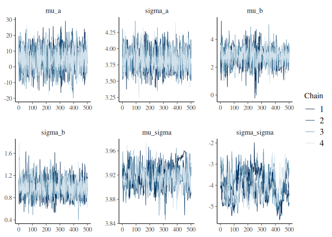
The traceplots and the summary statistics do show kind of the same story. The sigma_sigma and mu_sigma parameters are quite badly converged!
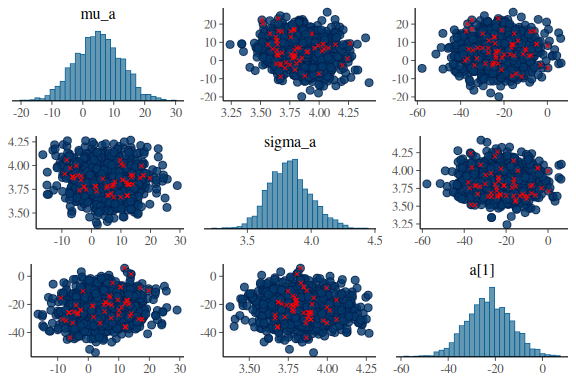
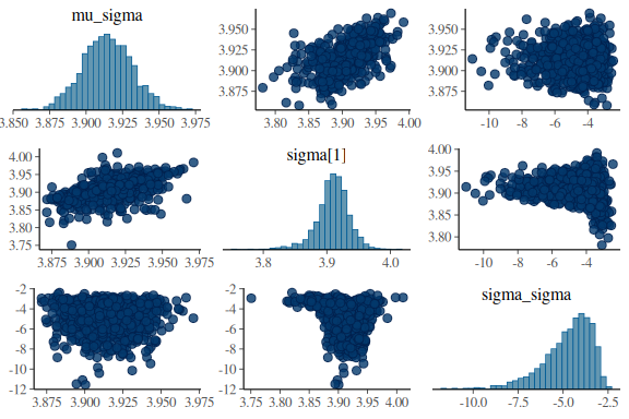
Now we’ll look at another diagnostic tool, the pair plots.
The is a plot with marginial histograms but also with pairwise scatterplots of the parameters. Additionally this function takes the information of the diagnoistics “np” and shows you which values got a divergences!
For the intercept:
mcmc_pairs(fit$draws(c("mu_a","sigma_a","a[1]")),
           np = nuts_params(fit))
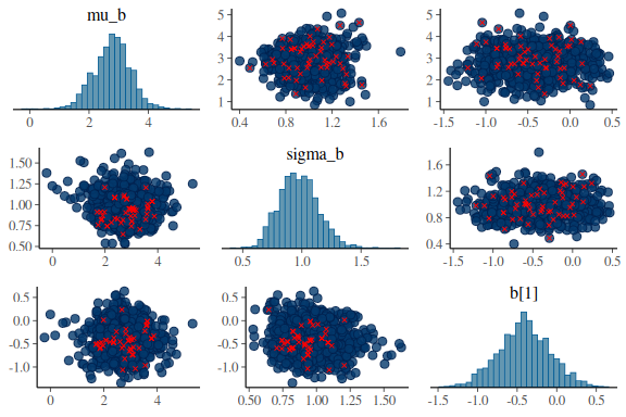
for the slope
mcmc_pairs(fit$draws(c("mu_b","sigma_b","b[1]")),
           np = nuts_params(fit))
for the standard deviation of the normal distribution
mcmc_pairs(fit$draws(c("mu_sigma","sigma[1]","sigma_sigma")),
           np = nuts_params(fit))
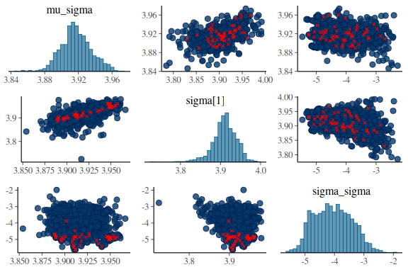
What one wants to see ideally in these plots is one big “blob” of points for all the pairwise scatter plots and histograms that are somewhat nicely normal. When we high the divergent transitions with red crosses and we see a pattern in where they are, they can give us clues into what the issue might be. The problem here is especially for the last plot of sigma and between the indidvidual sigma parameters (sigma[1]) and the standard deviations of the group level standard devivation (sigma_sigma). The pairwise scatter plot between these two shows a pattern where all the divergences are when sigma_sigma is low (below -4). This means that the sampler encounters issues in excatly that region and we thus need to help it!
This is probably the most common issue with hierarchical models. In more severe cases this behaviour will look like a funnel see plot from this awesome blog.
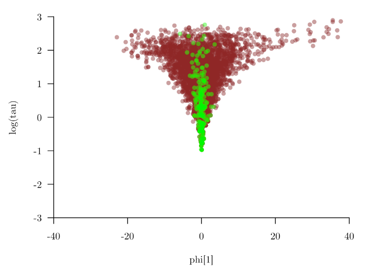
Fortunatly this problem has a quite easy solution, and has to do with parameterization as mentioned in the diagnoistics markdown. The solution is called non-centered parameterization.
Parameterization as mentioned refers to the way that the model is structured. Essentially there is many different ways of writing the same model, mathematically, and it turns our that some models are much easier to make converge with a particular way of writing the model.
What we have to do here is we need to re-write how we get our subject level parameters, instead of:
we will write it as:
which is mathematically equivalent.
What this essentially does, is that it makes us sample from a standard normal distribution which is going to be the subject level scaled difference between the group mean and subject.
Please note that i introduced another block which we will be using in later markdowns, the transformed parameters{…} block. Essentially this does nothing for the sample, but makes extracting the subject level parameters afterwards easier. We’ll get back to this block later on!
//This block defines the input that. So these things needs to go into the model
data {

  //Define the number of datapoints this is defined by an integer
  int N;

  //Define the number of subjects this is defined by an integer
  int S;

  //identifier for which subject this trial belongs to
  array[N] int  S_id;

  //Define a vector called y that is as long as the number of datapoints (i.e. N)
  vector[N] y;
  // same as y but a variable called x our independent variable
  vector[N] x;
}

// This is the parameters block.
// Here we define the free parameters which are the onces that STAN estimates for us.
// this is again a,b and sigma
parameters {
  real mu_a;
  real sigma_a;

  vector[S] a_dif;

  real mu_b;
  real sigma_b;

  vector[S] b_dif;

  real mu_sigma;
  real sigma_sigma;

  vector[S] sigma_dif;

}

// This is the model block here we define the model.

transformed parameters{

  vector[S] a = mu_a+a_dif*exp(sigma_a);
  vector[S] b = mu_b+b_dif*exp(sigma_b);
  vector[S] sigma = mu_sigma+sigma_dif*exp(sigma_sigma);

}

model {


  //priors
  mu_a ~ normal(0,10);
  sigma_a ~ normal(0,5);
  a_dif ~ std_normal();


  mu_b ~ normal(0,10);
  sigma_b ~ normal(0,5);

  b_dif ~ std_normal();


  mu_sigma ~ normal(0,3);
  sigma_sigma ~ normal(0,3);

  sigma_dif ~ std_normal();


  for(n in 1:N){

    y[n] ~ normal(a[S_id[n]]+b[S_id[n]]*x[n], exp(sigma[S_id[n]]));

  }
}
Note, I’ve set this chunk to message=FALSE which means no output is generated as there is a lot of warnings that are not important here.
# fit the model to the subsetted data
fit = model_obj2$sample(data = list(N = nrow(df), x = df$x,
                                    y = df$y_pred,
                                    S = length(unique(df$id)),
                                    S_id = df$id),
                        seed = seeds,
                        refresh = 500,
                        iter_warmup = 500,
                        iter_sampling = 500,
                        parallel_chains = 4)
## Running MCMC with 4 parallel chains...
##
## Chain 1 Iteration:   1 / 1000 [  0%]  (Warmup)
## Chain 2 Iteration:   1 / 1000 [  0%]  (Warmup)

## Chain 3 Iteration:   1 / 1000 [  0%]  (Warmup)

## Chain 4 Iteration:   1 / 1000 [  0%]  (Warmup)

## Chain 3 Iteration: 500 / 1000 [ 50%]  (Warmup)
## Chain 3 Iteration: 501 / 1000 [ 50%]  (Sampling)
## Chain 1 Iteration: 500 / 1000 [ 50%]  (Warmup)
## Chain 1 Iteration: 501 / 1000 [ 50%]  (Sampling)
## Chain 2 Iteration: 500 / 1000 [ 50%]  (Warmup)
## Chain 2 Iteration: 501 / 1000 [ 50%]  (Sampling)
## Chain 4 Iteration: 500 / 1000 [ 50%]  (Warmup)
## Chain 4 Iteration: 501 / 1000 [ 50%]  (Sampling)
## Chain 1 Iteration: 1000 / 1000 [100%]  (Sampling)
## Chain 1 finished in 18.2 seconds.
## Chain 4 Iteration: 1000 / 1000 [100%]  (Sampling)
## Chain 4 finished in 19.9 seconds.
## Chain 3 Iteration: 1000 / 1000 [100%]  (Sampling)
## Chain 3 finished in 21.2 seconds.
## Chain 2 Iteration: 1000 / 1000 [100%]  (Sampling)
## Chain 2 finished in 21.5 seconds.
##
## All 4 chains finished successfully.
## Mean chain execution time: 20.2 seconds.
## Total execution time: 21.5 seconds.
fit$diagnostic_summary()
## $num_divergent
## [1] 0 0 0 0
##
## $num_max_treedepth
## [1] 0 0 0 0
##
## $ebfmi
## [1] 0.7340319 0.8259069 0.7772488 0.7275951
Nothing from the sampler on diagnostics.
lets look at the summary and the trace plots for the group level parameters:
fit$summary(c("mu_a","sigma_a",
                       "mu_b","sigma_b",
                       "mu_sigma","sigma_sigma"))
## # A tibble: 6 × 10
##   variable      mean median     sd    mad     q5   q95  rhat ess_bulk ess_tail
##   <chr>        <dbl>  <dbl>  <dbl>  <dbl>  <dbl> <dbl> <dbl>    <dbl>    <dbl>
## 1 mu_a         4.83   5.00  7.73   7.34   -8.48  17.4   1.01     363.     657.
## 2 sigma_a      3.85   3.83  0.172  0.166   3.58   4.15  1.01     380.     641.
## 3 mu_b         2.71   2.67  0.654  0.640   1.67   3.83  1.02     163.     285.
## 4 sigma_b      0.973  0.957 0.169  0.160   0.720  1.28  1.00     361.     723.
## 5 mu_sigma     3.91   3.91  0.0169 0.0173  3.89   3.94  1.00    2944.    1395.
## 6 sigma_sigma -4.75  -4.47  1.36   1.24   -7.35  -3.07  1.00     968.    1051.
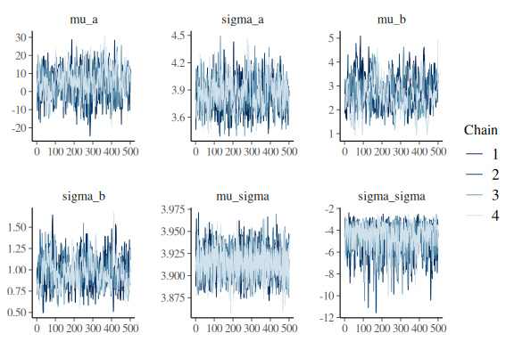
mcmc_trace(fit$draws(c("mu_a","sigma_a",
                       "mu_b","sigma_b",
                       "mu_sigma","sigma_sigma")))
And for good measure the pairplots.
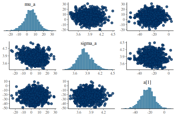
For the intercept:
mcmc_pairs(fit$draws(c("mu_a","sigma_a","a[1]")),
           np = nuts_params(fit))
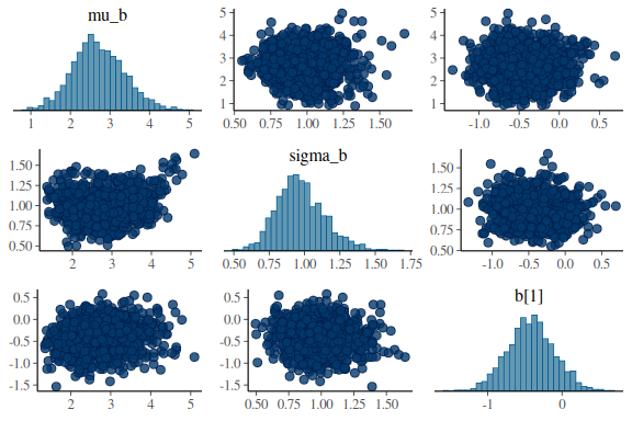
for the slope
mcmc_pairs(fit$draws(c("mu_b","sigma_b","b[1]")),
           np = nuts_params(fit))
for the standard deviation of the normal distribution
mcmc_pairs(fit$draws(c("mu_sigma","sigma[1]","sigma_sigma")),
           np = nuts_params(fit))
everything looks much better! Not perfect, but better and no divergences. Also Note that now the sampler as also moved all the way down into -12 in the sigma_sigma parameter, where before it only got to around ~ -5
Lets plot the group level predictions of this model.
Here we plot some of the draws as in the other markdowns:
group_draws = as_draws_df(fit$draws(c("mu_a","sigma_a",
                                      "mu_b","sigma_b",
                                      "mu_sigma","sigma_sigma")))

#get 200 random ids for the draws we select to plot.
draw_id = sample(1:4000,200)


params = group_draws %>% select(-contains(".")) %>%
  mutate(draw = 1:n()) %>%
  filter(draw %in% draw_id) %>%
  mutate(x = list(seq(0,50,length.out = n_trials))) %>%
  unnest(x) %>%
  rowwise() %>%
  mutate(y_mean = mu_a + mu_b * x)
## Warning: Dropping 'draws_df' class as required metadata was removed.
df %>% group_by(x) %>% summarize(mean = mean(y_pred), se = sd(y_pred)/sqrt(n())) %>%
  ggplot(aes(x = x, y = mean))+
  geom_line(data = params, aes(x = x, y = y_mean, group = draw), col = "red", alpha = 0.5)+
  geom_pointrange(aes(ymin = mean-2*se,ymax = mean+2*se))+
  theme_minimal()
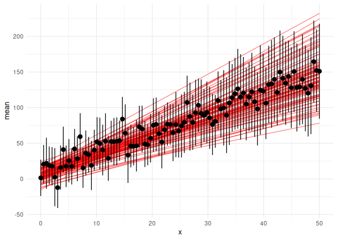
Looks really good!
Lets plot the individual subjects first just their mean predictions and data:
#get 50 random ids for the draws we select to plot.
draw_id = sample(1:4000,50)

subject_draws = as_draws_df(fit$draws(c("a","b","sigma"))) %>%
  select(-contains("."))
## Warning: Dropping 'draws_df' class as required metadata was removed.
params = subject_draws %>%
  mutate(draw = 1:n()) %>%
  filter(draw %in% draw_id) %>%
  pivot_longer(-draw) %>%
  mutate(
    # Extract the number in square brackets
    id = as.numeric(str_extract(name, "(?<=\\[)\\d+(?=\\])")),
    # Remove the number in square brackets from the name
    parameter = str_replace(name, "\\[([0-9]+)\\]", ""),
    name = NULL
  )%>%
  pivot_wider(names_from = "parameter", values_from = value) %>%
  group_by(draw,id) %>%
  mutate(x = list(seq(0,50,length.out = n_trials))) %>%
  unnest(x) %>%
  rowwise() %>%
  mutate(y_mean = a + b * x,
         y_pred_low = a+b*x - 2 * exp(sigma),
         y_pred_high = a+b*x + 2 * exp(sigma))


df %>% mutate(draw = NA) %>%
  ggplot(aes(x = x, y = y_pred,group = interaction(id,draw)))+
  geom_point()+
  geom_line(data = params, aes(x = x, y = y_mean), col = "red", alpha = 0.25)+
  facet_wrap(~id)+
  theme_minimal()
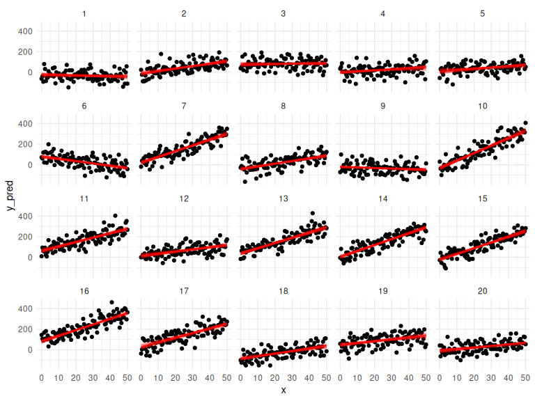
And their prediction intervals:
df %>% mutate(draw = NA) %>%
  ggplot()+
  geom_point(aes(x = x, y = y_pred,group = interaction(id,draw)))+
  geom_line(data = params, aes(x = x, y = y_mean, group = interaction(id,draw)), col = "red", alpha = 0.25)+
  geom_ribbon(data = params, aes(x = x, ymin = y_pred_low, ymax = y_pred_high), fill = "grey", alpha = 0.5)+
  facet_wrap(~id)+
  theme_minimal()
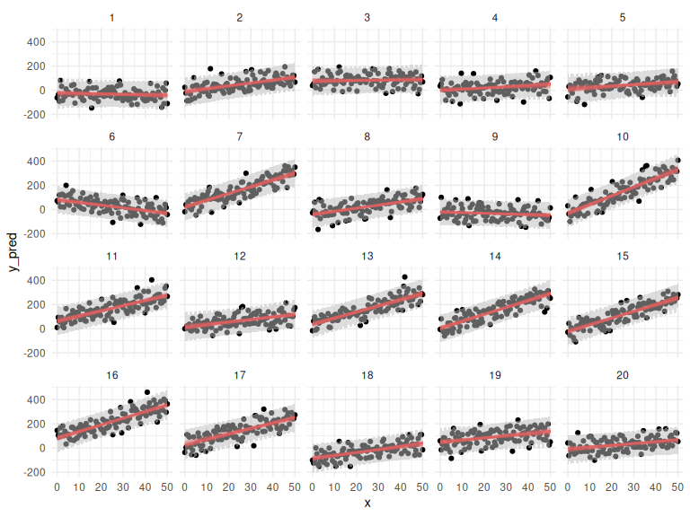
Not to bad either!
Final remarks
The main take aways are that hierarchical models are designed to fit subjects together in the same model, such that we leverage all the information and propergate all the uncertainty from subjects to get group level estimates. These types of models have become corner stones in the cognitive science literature, unfortunately they can be hard to estimate. The difficulty of estimation in the Bayesian framework is usually something that we can combat with clever use of priors and parameterizations (as shown here). Unfortunatly in the frequentists framework these models are sometimes impossible to fit due to bad convergences and one has to “strip down the random effects”. This pratice is essentially the same as saying that all subjects need to have the same group level slope above. This can lead to inflated type 1 error rates (ref?) and is generally not something I see positively.
Resources
Other really good resources can be found here.