
Multivariate Priors And Correlations
Published:
- Bayesian Workflow
This R introduces and expands on hierarchical modeling with variance co-variance matrices and multivariate distributions.
Table of content
- Overview
- Correlation coefficients.
- Simulations.
- Hierarchical modeling.
- Hierarchical modeling with correlations!
- Multivariate distributions inside stan.
- The LKJ distribution.
- Final remarks
Overview
When doing hierarchical modeling, we usually model subjects nested within a population. This entails estimating the parameters of our model for each individual in our data-set, but also a group level parameter. This approach to modeling the nested structure of our data have some nice properties such as partial pooling (Need to find a nice reference here). This aspect of hierarchical modeling essentially pools the individual subject estimates towards the group mean, because they are assumed to be drawn from this group mean distribution.
Another thing that is less commonly taught or talked about is that in hierarchical modeling is the correlation between the subject level parameters.
Correlation coefficients.
There exists many correlation coefficients including pearsons, spearman and kendells tau. In this section we are only interested in Pearsons correlation coefficients as it is what naturally comes out of a multivariate normal distribution (which is the multiivariate distribution I will be using).
Before diving into multivariate distribution we look at the standard formula for the Pearsons correlation coefficient.
where and
are the mean of the first and second variable respectively.
This can also be writing as covariance and variance in the following way, which will be helpful in a bit:
This is interesting as all of these entities are things that come out of a multivariate normal distribution, in the variance co-variance matrix (the last part below).
The way to understand this formula is that X and Y are the random variables (just as for the uni-variate case: e.g ). The first vector inside the normal distribution is the two means of the random variables
and
. The last part is the variance co-variance matrix which contains the variances of the random variables (squared standard deviatations from the uni-variate case e.g. (
)), but also the covariance between the random variables Cov(X,Y). These co-variances contains the information we need to compute the correlation coefficient together with the variances (eq. 1)
Lets demonstrate this by simulating some data
Simulations.
Below I will simulate from a multivariate normal with means of 0 and variances (and also standard deviations) 1.
This means that the off-diagonal (the Cov(X,Y) and Cov(Y,X)) of the variance-covariance matrix is the correlation coefficient (see this by setting the numerator to 1 in (1)). Thus here the correlation coefficient (and the covariance) is 0.5.
#data points
n <- 100
#variance co-variance matrix
R <- matrix(c(1, 0.5,
              0.5, 1),
            nrow = 2, ncol = 2, byrow = TRUE)
#means
mu <- c(X = 0, Y = 0)
#random variables from the multivariate normal
data = data.frame(mvtnorm::rmvnorm(n, mean = mu, sigma = R))
plotting it!
data %>%
  ggplot(aes(x = X, y = Y))+
  geom_point()+
  theme_minimal()
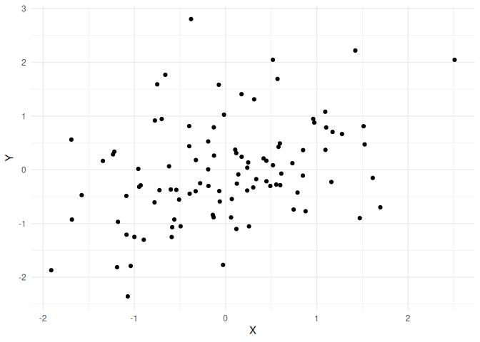
We see that there is a correlation which is around 0.5.
Hierarchical modeling.
There might be a couple of reasons to use multivariate distributions when doing hierarchical modeling. The first is that instead of assuming that all your parameters are independent, one lets the model estimate the correlation between them. This from practical experience gives close to the same estimates as just fitting these parameters independently and afterwards correlating them, thus this first aspect is just for convenience (not having to calculate the correlation coefficients afterwards).
The second reason for including multivariate distributions when doing hierarchical modeling has to do with generating data that would be expected from an experiment.
many times when simulating data from a hierarchical model we end up in a situations where we cannot achieve the behavior we expect from our real subjects. This is especially the case with more and more complex models (models with many parameters). The reason (sometimes) for this is that without dependency / correlations between the parameters the model will many times produce impossible or unreasonable data. Thus in order to simulate data that resemble what we expect we need to understand these correlations. In the following we will be doing this with a multivariate normal distribution, which means we need to assume that our priors for our parameters are all multi-variate normally distributed (another reason to have parameters be normally distributed and then transformed instead of coming from another distribtuion).
Hierarchical modeling with correlations!
Now we take the knowledge of simulations of multivariate normal distributions from above and apply it in the example used in the hierarchical modeling.
What needs to be stressed is that our individual data-points are going to be extracted exactly the same the only thing that changes is how we get the subject level parameters. We start with the simulation from before:
#number of simulated subjects
n_sub = 50
#number of simulated trials
n_trials = 100

#intercepts:
int = rnorm(n_sub,0,50)
#slopes:
slopes = rnorm(n_sub,3,3)
#sigma
sigma = 50

#x values
xs = seq(0,50,length.out = n_trials)

# simulate trialwise responses:
df_uncor = data.frame(intercept = int, slopes = slopes,sigma = sigma) %>%
  mutate(id = 1:n_sub,
         x = list(seq(0,50,length.out = n_trials))) %>%
  unnest(x) %>% rowwise() %>%
  mutate(y_mean = intercept + x * slopes,
         y_pred = rnorm(1,intercept + x * slopes, sigma))
Here we simulate 50 subjects of 100 trials each. Each subjects gets an intercept from the group level distribution of and a slope estimate from the same group level distribution of
.
Here we essentially fix group mean of the intercept to 0, and the between subject variance of the intercept to 50, whereas the group mean slope is 3 and the between subject variance of the slope to 3, and importantly with no correlation between the intercept and slope.
Now below we use the same values for means and standard deviations, but we sample the intercept and slope from the same multivariate normal distribution with a correlation of -0.8.
This correlation entails back-calculating the covariance from (1). which entails:
Simulating the data:
#number of simulated subjects
n_sub = 50
#number of simulated trials
n_trials = 100

mu_slope = 3
sd_slope = 3

mu_int = 0
sd_int= 50

correlation = -0.8

cov = correlation * sqrt(sd_slope^2 * sd_int ^2)

#variance co-variance matrix
R <- matrix(c(sd_int^2, cov,
              cov, sd_slope^2),
            nrow = 2, ncol = 2, byrow = TRUE)
#means
mu <- c(X = mu_int, Y = mu_slope)
#random variables from the multivariate normal
data = data.frame(mvtnorm::rmvnorm(n_sub, mean = mu, sigma = R)) %>%
  rename(intercept = X, slopes = Y)


#sigma
sigma = 50

#x values
xs = seq(0,50,length.out = n_trials)

# simulate trialwise responses:
df_cor = data %>% mutate(sigma = sigma) %>%
  mutate(id = 1:n_sub,
         x = list(seq(0,50,length.out = n_trials))) %>%
  unnest(x) %>% rowwise() %>%
  mutate(y_mean = intercept + x * slopes,
         y_pred = rnorm(1,intercept + x * slopes, sigma))
Lets plot the two to see the difference!
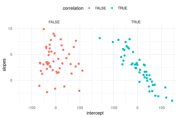
First on the parameters.
rbind(df_cor %>% mutate(correlation = T),df_uncor %>%
        mutate(correlation = F)) %>%
  dplyr::select(intercept, slopes,correlation) %>%
  ggplot(aes(x = intercept, y = slopes, col = correlation))+
  geom_point()+
  theme_minimal()+
  theme(legend.position = "top")+
  facet_wrap(~correlation)
And then the regression lines!
rbind(df_cor %>% mutate(correlation = T),
      df_uncor %>% mutate(correlation = F)) %>%
  ggplot(aes(x = x, y = y_mean,group = interaction(id,correlation), col = correlation))+
  geom_line()+
  theme_minimal()+facet_wrap(~correlation)
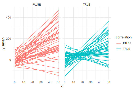
From these plots we see that the high negative correlation constrains the possible simulated values, such that the predicted mean responses are less spread out. This is because as the intercept becomes more positive the slopes have to becomes more negative and vise versa.
We can fit this using the same hierarchical model from before:
//This block defines the input that. So these things needs to go into the model
data {

  //Define the number of datapoints this is defined by an integer
  int N;

  //Define the number of subjects this is defined by an integer
  int S;

  //identifier for which subject this trial belongs to
  array[N] int  S_id;

  //Define a vector called y that is as long as the number of datapoints (i.e. N)
  vector[N] y;
  // same as y but a variable called x our independent variable
  vector[N] x;
}

// This is the parameters block.
// Here we define the free parameters which are the onces that STAN estimates for us.
// this is again a,b and sigma
parameters {
  real mu_a;
  real sigma_a;

  vector[S] a_dif;

  real mu_b;
  real sigma_b;

  vector[S] b_dif;

  real mu_sigma;
  real sigma_sigma;

  vector[S] sigma_dif;

}

// This is the model block here we the model.

transformed parameters{

  vector[S] a = mu_a+a_dif*exp(sigma_a);
  vector[S] b = mu_b+b_dif*exp(sigma_b);
  vector[S] sigma = mu_sigma+sigma_dif*exp(sigma_sigma);

}

model {

  //priors
  mu_a ~ normal(0,10);
  sigma_a ~ normal(0,5);
  a_dif ~ std_normal();


  mu_b ~ normal(0,10);
  sigma_b ~ normal(0,5);

  b_dif ~ std_normal();


  mu_sigma ~ normal(0,3);
  sigma_sigma ~ normal(0,3);

  sigma_dif ~ std_normal();

  for(n in 1:N){

    y[n] ~ normal(a[S_id[n]]+b[S_id[n]]*x[n], exp(sigma[S_id[n]]));

  }
}
Note, I’ve set this chunk to message=FALSE which means no output is generated as there is a lot of warnings that are not important here.
# fit the model to the subsetted data
fit = model_obj2$sample(data = list(N = nrow(df_cor), x = df_cor$x,
                                    y = df_cor$y_pred,
                                    S = length(unique(df_cor$id)),
                                    S_id = df_cor$id),
                        seed = seeds,
                        #warm-up samples
                        iter_warmup = 500,
                        #inference samples
                        iter_sampling = 500,
                        #chains
                        chains = 4,
                        #parallel chains
                        parallel_chains = 4,
                        #refresh rate of printing
                        refresh = 250,
                        #adap delta argument default 0.9
                        adapt_delta = 0.9)
## Running MCMC with 4 parallel chains...
##
## Chain 1 Iteration:   1 / 1000 [  0%]  (Warmup)

## Chain 2 Iteration:   1 / 1000 [  0%]  (Warmup)
## Chain 3 Iteration:   1 / 1000 [  0%]  (Warmup)

## Chain 4 Iteration:   1 / 1000 [  0%]  (Warmup)

## Chain 2 Iteration: 250 / 1000 [ 25%]  (Warmup)
## Chain 3 Iteration: 250 / 1000 [ 25%]  (Warmup)
## Chain 4 Iteration: 250 / 1000 [ 25%]  (Warmup)
## Chain 1 Iteration: 250 / 1000 [ 25%]  (Warmup)
## Chain 2 Iteration: 500 / 1000 [ 50%]  (Warmup)
## Chain 2 Iteration: 501 / 1000 [ 50%]  (Sampling)
## Chain 3 Iteration: 500 / 1000 [ 50%]  (Warmup)
## Chain 3 Iteration: 501 / 1000 [ 50%]  (Sampling)
## Chain 1 Iteration: 500 / 1000 [ 50%]  (Warmup)
## Chain 1 Iteration: 501 / 1000 [ 50%]  (Sampling)
## Chain 4 Iteration: 500 / 1000 [ 50%]  (Warmup)
## Chain 4 Iteration: 501 / 1000 [ 50%]  (Sampling)
## Chain 2 Iteration: 750 / 1000 [ 75%]  (Sampling)
## Chain 1 Iteration: 750 / 1000 [ 75%]  (Sampling)
## Chain 3 Iteration: 750 / 1000 [ 75%]  (Sampling)
## Chain 2 Iteration: 1000 / 1000 [100%]  (Sampling)
## Chain 2 finished in 70.4 seconds.
## Chain 4 Iteration: 750 / 1000 [ 75%]  (Sampling)
## Chain 1 Iteration: 1000 / 1000 [100%]  (Sampling)
## Chain 1 finished in 77.8 seconds.
## Chain 3 Iteration: 1000 / 1000 [100%]  (Sampling)
## Chain 3 finished in 86.2 seconds.
## Chain 4 Iteration: 1000 / 1000 [100%]  (Sampling)
## Chain 4 finished in 86.4 seconds.
##
## All 4 chains finished successfully.
## Mean chain execution time: 80.2 seconds.
## Total execution time: 86.7 seconds.
fit$diagnostic_summary()
## $num_divergent
## [1] 0 0 0 0
##
## $num_max_treedepth
## [1] 0 0 0 0
##
## $ebfmi
## [1] 0.7874689 0.8137758 0.7515242 0.7521037
Looks to fit nicely, but less go through the motions:
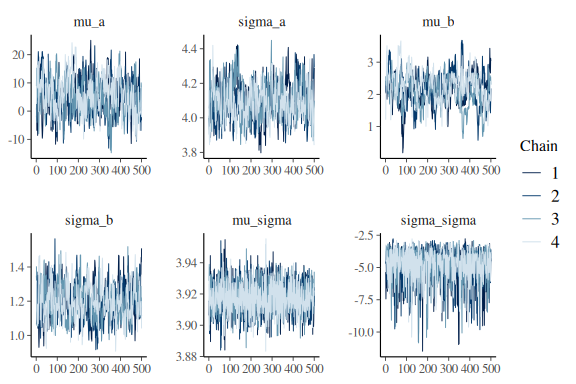
lets look at the summary and the trace plots for the group level parameters:
fit$summary(c("mu_a","sigma_a",
                       "mu_b","sigma_b",
                       "mu_sigma","sigma_sigma"))
## # A tibble: 6 × 10
##   variable     mean median     sd     mad    q5   q95  rhat ess_bulk ess_tail
##   <chr>       <dbl>  <dbl>  <dbl>   <dbl> <dbl> <dbl> <dbl>    <dbl>    <dbl>
## 1 mu_a         5.38   5.29 6.29   6.19    -4.92 16.1   1.01     219.     511.
## 2 sigma_a      4.10   4.10 0.103  0.103    3.93  4.27  1.02     285.     503.
## 3 mu_b         2.16   2.18 0.481  0.475    1.37  2.88  1.03     114.     282.
## 4 sigma_b      1.20   1.19 0.102  0.105    1.04  1.37  1.01     345.     805.
## 5 mu_sigma     3.92   3.92 0.0100 0.00981  3.90  3.93  1.00    3887.    1555.
## 6 sigma_sigma -4.98  -4.70 1.33   1.15    -7.57 -3.34  1.00    1045.    1189.
mcmc_trace(fit$draws(c("mu_a","sigma_a",
                       "mu_b","sigma_b",
                       "mu_sigma","sigma_sigma")))
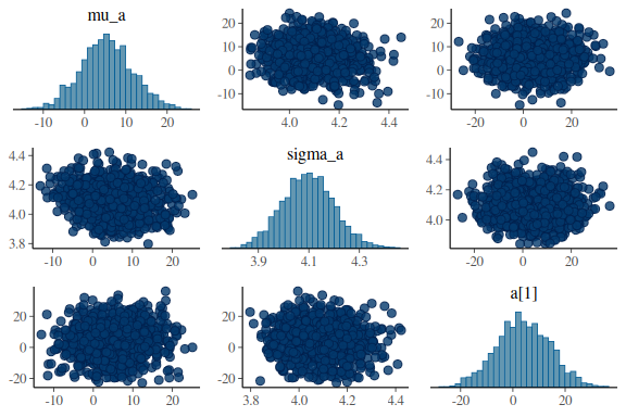
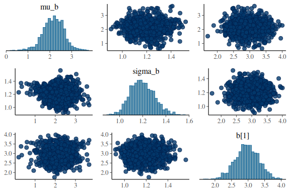
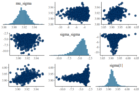
And for good measure the pairplots
mcmc_pairs(fit$draws(c("mu_a","sigma_a","a[1]")),
           np = nuts_params(fit))
mcmc_pairs(fit$draws(c("mu_b","sigma_b","b[1]")),
           np = nuts_params(fit))
mcmc_pairs(fit$draws(c("mu_sigma","sigma_sigma","sigma[1]")),
           np = nuts_params(fit))
Now also the posterior predictive checks:
group_draws = as_draws_df(fit$draws(c("mu_a","sigma_a",
                                      "mu_b","sigma_b",
                                      "mu_sigma","sigma_sigma")))

#get 200 random ids for the draws we select to plot.
draw_id = sample(1:4000,200)


params = group_draws %>% dplyr::select(-contains(".")) %>%
  mutate(draw = 1:n()) %>%
  filter(draw %in% draw_id) %>%
  mutate(x = list(seq(0,50,length.out = n_trials))) %>%
  unnest(x) %>%
  rowwise() %>%
  mutate(y_mean = mu_a + mu_b * x)
## Warning: Dropping 'draws_df' class as required metadata was removed.
df_cor %>% group_by(x) %>% summarize(mean = mean(y_pred),
                                     se = sd(y_pred)/sqrt(n())) %>%
  ggplot(aes(x = x, y = mean))+
  geom_line(data = params, aes(x = x, y = y_mean, group = draw), col = "red", alpha = 0.5)+
  geom_pointrange(aes(ymin = mean-2*se,ymax = mean+2*se))+
  theme_minimal()
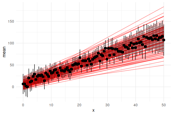
Looks really good!
Lets plot the indivudal subjects:
#get 50 random ids for the draws we select to plot.
draw_id = sample(1:4000,50)

subject_draws = as_draws_df(fit$draws(c("a","b","sigma"))) %>%
  dplyr::select(-contains("."))
## Warning: Dropping 'draws_df' class as required metadata was removed.
params = subject_draws %>%
mutate(draw = 1:n()) %>%
filter(draw %in% draw_id) %>%
pivot_longer(-draw) %>%
mutate(
# Extract the number in square brackets
id = as.numeric(str_extract(name, "(?<=\\[)\\d+(?=\\])")),
# Remove the number in square brackets from the name
parameter = str_replace(name, "\\[([0-9]+)\\]", ""),
name = NULL
)%>%
pivot_wider(names_from = "parameter", values_from = value) %>%
group_by(draw,id) %>%
mutate(x = list(seq(0,50,length.out = n_trials))) %>%
unnest(x) %>%
rowwise() %>%
mutate(y_mean = a + b * x,
y_pred_low = a+b*x - 2 * exp(sigma),
y_pred_high = a+b*x + 2 * exp(sigma))
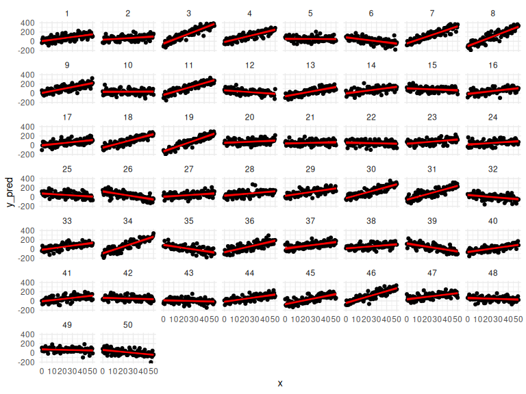
df_cor %>% mutate(draw = NA) %>%
ggplot(aes(x = x, y = y_pred,group = interaction(id,draw)))+
geom_point()+
geom_line(data = params, aes(x = x, y = y_mean), col = "red", alpha = 0.25)+
facet_wrap(~id)+
theme_minimal()
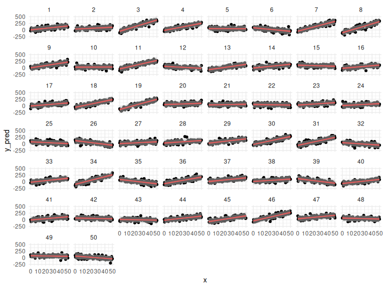
With prediction intervals:
df_cor %>% mutate(draw = NA) %>%
  ggplot()+
  geom_point(aes(x = x, y = y_pred,group = interaction(id,draw)))+
  geom_line(data = params, aes(x = x, y = y_mean, group = interaction(id,draw)), col = "red", alpha = 0.25)+
  geom_ribbon(data = params, aes(x = x, ymin = y_pred_low, ymax = y_pred_high), fill = "grey", alpha = 0.5)+
  facet_wrap(~id)+
  theme_minimal()
Also looks good! Lets calculate the correlation that stan find between the slope and the intercept!
To do this we get two data-frames one with the draws from the intercept for all subjects and one for the slopes:
subject_draws = as_draws_df(fit$draws(c("mu_b","sigma_b","b_dif"))) %>%
  dplyr::select(-contains("."))
## Warning: Dropping 'draws_df' class as required metadata was removed.
slope_draws = subject_draws %>%
  mutate(draw = 1:n()) %>%
  pivot_longer(
    cols = matches("^(a|b|sigma)_dif"),
    names_to = c("parameter", "id"),
    names_pattern = "(.*)_(dif\\[\\d+\\])"
  ) %>%
  mutate(id = str_extract(id, "\\d+")) %>%
  pivot_wider(names_from = "parameter", values_from = value) %>%
  mutate(b = mu_b + b * sigma_b) %>% dplyr::select(id,b) %>%
  pivot_wider(names_from = id, values_from = b) %>% unnest()
## Warning: Values from `b` are not uniquely identified; output will contain list-cols.
## • Use `values_fn = list` to suppress this warning.
## • Use `values_fn = {summary_fun}` to summarise duplicates.
## • Use the following dplyr code to identify duplicates.
##   {data} |>
##   dplyr::summarise(n = dplyr::n(), .by = c(id)) |>
##   dplyr::filter(n > 1L)

## Warning: `cols` is now required when using `unnest()`.
## ℹ Please use `cols = c(`1`, `2`, `3`, `4`, `5`, `6`, `7`, `8`, `9`, `10`, `11`,
##   `12`, `13`, `14`, `15`, `16`, `17`, `18`, `19`, `20`, `21`, `22`, `23`, `24`,
##   `25`, `26`, `27`, `28`, `29`, `30`, `31`, `32`, `33`, `34`, `35`, `36`, `37`,
##   `38`, `39`, `40`, `41`, `42`, `43`, `44`, `45`, `46`, `47`, `48`, `49`,
##   `50`)`.
subject_draws = as_draws_df(fit$draws(c("mu_a","sigma_a","a_dif"))) %>%
  dplyr::select(-contains("."))
## Warning: Dropping 'draws_df' class as required metadata was removed.
int_draws = subject_draws %>%
  mutate(draw = 1:n()) %>%
  pivot_longer(
    cols = matches("^(a|b|sigma)_dif"),
    names_to = c("parameter", "id"),
    names_pattern = "(.*)_(dif\\[\\d+\\])"
  ) %>%
  mutate(id = str_extract(id, "\\d+")) %>%
  pivot_wider(names_from = "parameter", values_from = value) %>%
  mutate(a = mu_a + a * sigma_a) %>% dplyr::select(id,a) %>%
  pivot_wider(names_from = id, values_from = a) %>% unnest()
## Warning: Values from `a` are not uniquely identified; output will contain list-cols.
## • Use `values_fn = list` to suppress this warning.
## • Use `values_fn = {summary_fun}` to summarise duplicates.
## • Use the following dplyr code to identify duplicates.
##   {data} |>
##   dplyr::summarise(n = dplyr::n(), .by = c(id)) |>
##   dplyr::filter(n > 1L)
## `cols` is now required when using `unnest()`.
## ℹ Please use `cols = c(`1`, `2`, `3`, `4`, `5`, `6`, `7`, `8`, `9`, `10`, `11`,
##   `12`, `13`, `14`, `15`, `16`, `17`, `18`, `19`, `20`, `21`, `22`, `23`, `24`,
##   `25`, `26`, `27`, `28`, `29`, `30`, `31`, `32`, `33`, `34`, `35`, `36`, `37`,
##   `38`, `39`, `40`, `41`, `42`, `43`, `44`, `45`, `46`, `47`, `48`, `49`,
##   `50`)`.
Then we make an empty vector where we store all the correlation coefficients when we loop through the draws: (this is very inefficient but works for now).
correlation_coef = c()
for(i in 1:2000){
  correlation_coef[i] = cor.test(as.numeric(slope_draws[i,]),
                                 as.numeric(int_draws[i,]))$estimate[[1]]
}
now we can plot the distribution of correlation coefficients:
data.frame() %>%
  ggplot(aes(x = correlation_coef))+
  geom_histogram(col = "black")+
  theme_minimal()+
  xlab("Correlation coefficient")
## `stat_bin()` using `bins = 30`. Pick better value with `binwidth`.
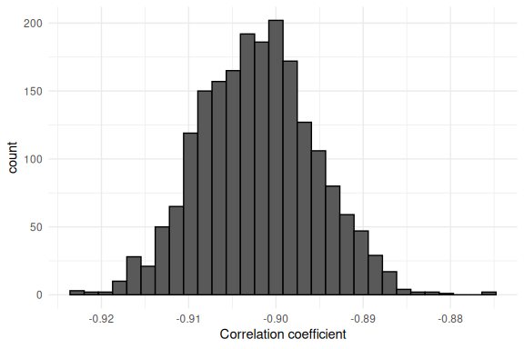
Now one might say “But hey we put in -0.8 didn’t we?”. This would be correct, however there is some uncertainty in this, so we can go back to the data and see what the correlation between the slope and intercept actually was:
parameters = df_cor %>% dplyr::select(intercept, slopes) %>%
  distinct()

cor.test(parameters$intercept,parameters$slopes)
##
##  Pearson's product-moment correlation
##
## data:  parameters$intercept and parameters$slopes
## t = -14.87, df = 48, p-value < 2.2e-16
## alternative hypothesis: true correlation is not equal to 0
## 95 percent confidence interval:
##  -0.9460860 -0.8400408
## sample estimates:
##        cor
## -0.9064413
-0.90 which is very close to what Stan gives out!
Multivariate distributions inside stan.
Now we have simulated data where the parameters had a correlation of ~0.8 and then fitted a Stan model without specifying the correlation coefficient, but still being able to estimate it. Thus one might ask whether it even makes sense to code the Stan model with the correlation coefficient.
I have no good reasons other than it being convenient to why one wants to calculate the correlation within Stan using multivariate normal distribution priors on the parameters. One small reason is that its possible (and necessary) to put a prior on the correlation coefficient. Below is how to do this inside Stan! Note; there are a couple of things different from the other Stan formulation! Some for ease and others that are crucial for the variance co-variance matrix.
Lets look at the differences between the two implementations:
group means and between subject variances (mu_* and sigma_*) are now stored in vectors called mus and sigmas respectively.
The subject level differences (the standard normal distribution for the non-centered parameterization) are now stored in a matrix of [N_params , subjects].
In the parameters block, another variable “L_u” is defined as a cholesky_factor_corr[3]. This thing is essentially what helps define the covariance (and therefore also the correlation) between the variables. This is a reparameterization (just as the non-centered parameterization) to help the sampler not run into sampling issues. For the example of not reparameterizing such a multivariate model (and therefore modeling the variance -covariance matrix directly) see the fantastic explanation on 11.1.3.
The start of the model block includes a new “transformed_difs” parameter that contains the subject level differences from the group means in a matrix with columns being the parameters (1 through 3) and the subjects being the rows. Is thus makes sense that each individual subject level parameter is defined afterwards as the group mean plus this difference.
Because we defined the new “L_u” parameter that contains the information about the correlation between our subject level parameters, we also need to add a prior on it. This is what the line “L_u ~ lkj_corr_cholesky(2);” does. To get a sense of what this distribtuion entails for the prior on the correlation coefficient, see the end of this markdown. Here it suffices to say that the 2 is a wide but not uniform distribution on the correlation coefficient within the constrained range of correlation coefficients [-1 ; 1].
Lastly, we use the last type of “block” in Stan, the generated quantities block. This block is outside of optimization, so all that happens here is based on the results of the fitted model and could in principle be done outside of Stan. In the generated quantities block we calculate the correlation matrix for convenience, which means that one can get the correlation matrix out using fit$summary(correlation_matrix), instead of doing the operation after model fitting.
//This block defines the input that. So these things needs to go into the model
data {

  //Define the number of datapoints this is defined by an integer
  int N;

  //Define the number of subjects this is defined by an integer
  int S;

  //identifier for which subject this trial belongs to
  array[N] int  S_id;

  //Define a vector called y that is as long as the number of datapoints (i.e. N)
  vector[N] y;
  // same as y but a variable called x our independent variable
  vector[N] x;
}

// This is the parameters block.
// Here we define the free parameters which are the onces that STAN estimates for us.
// this is again a,b and sigma
parameters {

  vector[3] mus;

  vector<lower=0>[3] sigmas;
  matrix[3,S] difs;
  cholesky_factor_corr[3] L_u;    // Between participant cholesky decomposition

}

// This is the model block here we define the model

model {
  matrix[S, 3] transformed_difs = (diag_pre_multiply(sigmas, L_u) * difs)'; // transformed deviations
  vector[S] a = mus[1] + (transformed_difs[,1]); // intercept per subject
  vector[S] b = mus[2] + (transformed_difs[,2]); // slope per subject
  vector[S] sigma = mus[3] + (transformed_difs[,3]); // standard deviation per subject


  //priors
  mus[1] ~ normal(0,10);
  sigmas[1] ~ normal(50,20);

  mus[2] ~ normal(0,10);
  sigmas[2] ~ normal(2,2);

  mus[3] ~ normal(0,3);
  sigmas[3] ~ normal(0,3);

  to_vector(difs) ~ std_normal();

  L_u ~ lkj_corr_cholesky(2);

  for(n in 1:N){

    y[n] ~ normal(a[S_id[n]]+b[S_id[n]]*x[n], exp(sigma[S_id[n]]));

  }
}

generated quantities{
  matrix[3,3] correlation_matrix = L_u * L_u';
}
Lets try and fit it!
Note, I’ve set this chunk to message=FALSE which means no output is generated as there is a lot of warnings that are not important here.
# fit the model to the subsetted data
fit = model_obj2$sample(data = list(N = nrow(df_cor), x = df_cor$x,
                                    y = df_cor$y_pred,
                                    S = length(unique(df_cor$id)),
                                    S_id = df_cor$id),
                        seed = seeds,
                        #warm-up samples
                        iter_warmup = 500,
                        #inference samples
                        iter_sampling = 500,
                        #chains
                        chains = 4,
                        #parallel chains
                        parallel_chains = 4,
                        #refresh rate of printing
                        refresh = 250,
                        #adap delta argument default 0.9
                        adapt_delta = 0.9)
## Running MCMC with 4 parallel chains...
##
## Chain 1 Iteration:   1 / 1000 [  0%]  (Warmup)

## Chain 2 Iteration:   1 / 1000 [  0%]  (Warmup)

## Chain 3 Iteration:   1 / 1000 [  0%]  (Warmup)

## Chain 4 Iteration:   1 / 1000 [  0%]  (Warmup)

## Chain 4 Iteration: 250 / 1000 [ 25%]  (Warmup)
## Chain 3 Iteration: 250 / 1000 [ 25%]  (Warmup)
## Chain 2 Iteration: 250 / 1000 [ 25%]  (Warmup)
## Chain 1 Iteration: 250 / 1000 [ 25%]  (Warmup)
## Chain 3 Iteration: 500 / 1000 [ 50%]  (Warmup)
## Chain 3 Iteration: 501 / 1000 [ 50%]  (Sampling)
## Chain 4 Iteration: 500 / 1000 [ 50%]  (Warmup)
## Chain 4 Iteration: 501 / 1000 [ 50%]  (Sampling)
## Chain 1 Iteration: 500 / 1000 [ 50%]  (Warmup)
## Chain 1 Iteration: 501 / 1000 [ 50%]  (Sampling)
## Chain 2 Iteration: 500 / 1000 [ 50%]  (Warmup)
## Chain 2 Iteration: 501 / 1000 [ 50%]  (Sampling)
## Chain 1 Iteration: 750 / 1000 [ 75%]  (Sampling)
## Chain 3 Iteration: 750 / 1000 [ 75%]  (Sampling)
## Chain 4 Iteration: 750 / 1000 [ 75%]  (Sampling)
## Chain 1 Iteration: 1000 / 1000 [100%]  (Sampling)
## Chain 1 finished in 74.8 seconds.
## Chain 2 Iteration: 750 / 1000 [ 75%]  (Sampling)
## Chain 3 Iteration: 1000 / 1000 [100%]  (Sampling)
## Chain 3 finished in 87.3 seconds.
## Chain 4 Iteration: 1000 / 1000 [100%]  (Sampling)
## Chain 4 finished in 88.5 seconds.
## Chain 2 Iteration: 1000 / 1000 [100%]  (Sampling)
## Chain 2 finished in 100.4 seconds.
##
## All 4 chains finished successfully.
## Mean chain execution time: 87.7 seconds.
## Total execution time: 100.6 seconds.
fit$diagnostic_summary()
## $num_divergent
## [1] 0 0 0 0
##
## $num_max_treedepth
## [1] 0 0 0 0
##
## $ebfmi
## [1] 0.8051629 0.7192983 0.6294704 0.8122553
Look at the summary, just to make sure the group level parameters have converged
fit
##   variable      mean    median    sd   mad        q5       q95 rhat ess_bulk
##  lp__      -22166.17 -22166.10 11.32 11.56 -22185.51 -22148.00 1.01      400
##  mus[1]         4.97      4.95  6.75  6.55     -6.28     16.02 1.02      209
##  mus[2]         2.41      2.42  0.40  0.41      1.79      3.05 1.01      243
##  mus[3]         3.92      3.92  0.01  0.01      3.90      3.93 1.00     3217
##  sigmas[1]     59.62     59.32  5.66  5.47     51.05     69.72 1.01      296
##  sigmas[2]      3.25      3.24  0.32  0.32      2.76      3.81 1.01      283
##  sigmas[3]      0.01      0.01  0.01  0.01      0.00      0.04 1.00      883
##  difs[1,1]     -0.03     -0.03  0.20  0.20     -0.36      0.30 1.00      633
##  difs[2,1]      0.34      0.34  0.23  0.23     -0.03      0.71 1.00      604
##  difs[3,1]      0.16      0.19  0.99  1.00     -1.43      1.73 1.00     3731
##  ess_tail
##       988
##       344
##       354
##      1616
##       510
##       476
##       849
##      1252
##       853
##      1429
##
##  # showing 10 of 175 rows (change via 'max_rows' argument or 'cmdstanr_max_rows' option)
We can now check the correlation matrix.
Here just the summary.
fit$summary("correlation_matrix")
## # A tibble: 9 × 10
##   variable       mean median     sd    mad     q5    q95  rhat ess_bulk ess_tail
##   <chr>         <dbl>  <dbl>  <dbl>  <dbl>  <dbl>  <dbl> <dbl>    <dbl>    <dbl>
## 1 correlation…  1      1     0      0       1      1     NA         NA       NA
## 2 correlation… -0.889 -0.892 0.0300 0.0274 -0.932 -0.833  1.02     367.     425.
## 3 correlation…  0.110  0.125 0.376  0.403  -0.534  0.706  1.00    2834.     959.
## 4 correlation… -0.889 -0.892 0.0300 0.0274 -0.932 -0.833  1.02     367.     425.
## 5 correlation…  1      1     0      0       1      1     NA         NA       NA
## 6 correlation… -0.112 -0.124 0.376  0.392  -0.712  0.543  1.00    2860.    1298.
## 7 correlation…  0.110  0.125 0.376  0.403  -0.534  0.706  1.00    2834.     959.
## 8 correlation… -0.112 -0.124 0.376  0.392  -0.712  0.543  1.00    2860.    1298.
## 9 correlation…  1      1     0      0       1      1     NA         NA       NA
Here the correlation that we care about (the one we put in) is the one with rows and columns of [2,1] or [1,2] (as its symmetrical).
Which is again basically what the simulation showed of -0.9
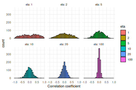
The LKJ distribution.
Below i plot a couple of values of the LKJ distribution for 3 parameters. The random number generator for this distribution can be found in the ggdist package.
Note; the function takes 3 arguments. Number of samples, number of parameters and the eta-value which i show below is the precision around
- Higher values of eta is equal to less probability in the extreme correlations.
etas = c(1,2,5,10,20,100)

df = data.frame()
for(eta in etas){
  draws = ggdist::rlkjcorr_marginal(1000,3,eta)
  dq = data.frame(draws = draws, eta = eta)
  df = rbind(df,dq)
}

df %>% mutate(eta = as.factor(eta)) %>%
  ggplot(aes(x = draws, fill = eta))+
  geom_histogram(col = "black", position = "identity")+
  theme_minimal()+
  facet_wrap(~eta, labeller = label_both)+
  xlab("Correlation coefficient")
## `stat_bin()` using `bins = 30`. Pick better value with `binwidth`.
Final remarks
In this markdown we have look at multivariate prior distributions for our hierarchical models and the subject level parameters in these. It should be clear from the markdown that incorporating the multivariate priors is not necessary for correct inference on the parameters and their correlations, but just a convenience! The main part to take away from this markdown is the simulations of correlated parameters. This will become quite important when wanting to simulate data that could come from an experimental paradigm. If non-correlated parameters (independent priors) are simulated the response profiles will be very wide and thus unreasonable. For additional context watch this Youtube video of Paul Bürkner.