Parameter Recovery

19 minute read

Published: January 06, 2025

Bayesian Workflow

This R markdown is for conducting parameter recovery.

Table of content

Overview
fitting a single model:
Extracting information from the posterior
Furrr and parallelization
Final remarks
SBC references

Overview

Here we combine the knowledge from the previous 4 markdowns (1 through 4) to conduct a parameter recovery analysis. The idea with parameter recovery is that we want to fit our Stan model to many simulated data-sets across many different combinations of parameter values. The goal here will be to plot simulated parameter values against estimated parameter values. As an additional step I will also highlight why the number of trials in the simulation matters.

Thus, what we aim to do in this markdown is setup scripts that let us generalize simulating, fitting and check diagnostics across parameter and trial values. Given the previous markdowns we will here demonstrate parameter recovery using the psychometric function that we simulated data from in the data simulation markdown and fitted in the diagnoistics.

A short reminder of the psychometric model; We assume that agents get a “stimulus” value (x) that they give a binary choice (y) to. This binary choice stems from a probability that is dependent on the stimulus and tree subject level parameters $\alpha$ (threshold), $\beta$ (slope) and $\lambda$ (lapse rate), that govern the shape of the psychometric.

Starting by simulating a single agent

#data points
N = 100
#threshold
alpha = 20
#slope
beta = 3

#lapse
lambda = 0.05

#x's
x = seq(-20,40, length.out = N)

# getting the probabilities from the model and the parameters
p = lambda+(1-2*lambda)*(0.5+0.5*pracma::erf((x-alpha)/(sqrt(2)*beta)))

And plotting it

data.frame() %>% ggplot(aes(x =x,y = p))+geom_point()+theme_classic()

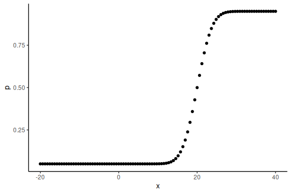
These are the latent probabilities that we wont see when we would get experimental data.

We would only see the realization of these (i.e the binary choice).

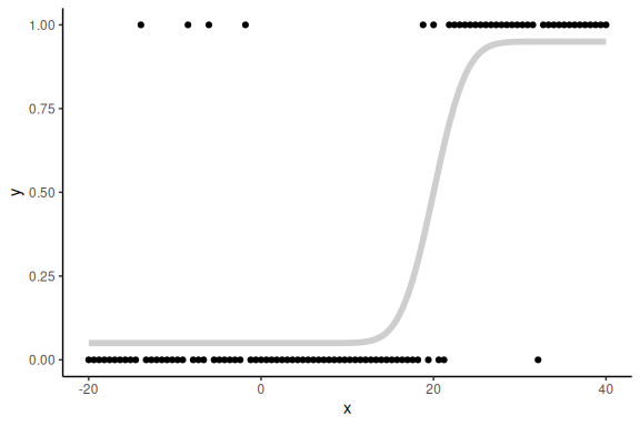
Plotting both:

# generating binary responses from the probabilities above
y = rbinom(N,1,p)

data.frame() %>% ggplot(aes(x =x,y = y))+
  geom_point()+
  theme_classic()+
  geom_line(aes(x = x, y = p), col = "grey", alpha = 0.75, linewidth = 2)

fitting a single model:

Using the same model as in the diagnostic markdown (with the “thight priors”):

//This block defines the input that. So these things needs to go into the model
data {
  //Define the number of datapoints this is defined by an integer
  int N;
  //Define an array called y that is as long as the number of datapoints (i.e. N) (Note these are integers)
  array[N] int y;
  // same as y but a variable called x our independent variable
  vector[N] x;
}

// This is the parameters block. 
// Here we define the free parameters which are the onces that STAN estimates for us.
// this is again a,b and sigma
parameters {
  real alpha;
  real beta;
  real lambda;
}

// This is the model block here we define the model.

model {
  //priors for the model
  alpha ~ normal(10,20);
  beta ~ normal(0,2);
  lambda ~ normal(-4,2);
  
  y ~ bernoulli(inv_logit(lambda)/2+(1-2*inv_logit(lambda)/2)*(0.5+0.5*erf((x-alpha)/(sqrt(2)*exp(beta)))));
}

Now we fit the model to the data by entering our data:

# Fit the STAN model
fit = model_obj2$sample(data = list(N =N, x = x, y =y),
                         seed = seeds,
                        #warm-up samples
                        iter_warmup = 500,
                        #inference samples
                        iter_sampling = 500,
                        #chains
                        chains = 4,
                        #parallel chains
                        parallel_chains = 4,
                        #refresh rate of printing
                        refresh = 250,
                        #adap delta argument default 0.9
                        adapt_delta = 0.9)

## Running MCMC with 4 parallel chains...
## 
## Chain 1 Iteration:   1 / 1000 [  0%]  (Warmup) 
## Chain 1 Iteration: 250 / 1000 [ 25%]  (Warmup) 
## Chain 1 Iteration: 500 / 1000 [ 50%]  (Warmup) 
## Chain 1 Iteration: 501 / 1000 [ 50%]  (Sampling) 
## Chain 1 Iteration: 750 / 1000 [ 75%]  (Sampling) 
## Chain 1 Iteration: 1000 / 1000 [100%]  (Sampling) 
## Chain 2 Iteration:   1 / 1000 [  0%]  (Warmup) 
## Chain 2 Iteration: 250 / 1000 [ 25%]  (Warmup) 
## Chain 2 Iteration: 500 / 1000 [ 50%]  (Warmup) 
## Chain 2 Iteration: 501 / 1000 [ 50%]  (Sampling) 
## Chain 2 Iteration: 750 / 1000 [ 75%]  (Sampling) 
## Chain 2 Iteration: 1000 / 1000 [100%]  (Sampling) 
## Chain 3 Iteration:   1 / 1000 [  0%]  (Warmup) 
## Chain 3 Iteration: 250 / 1000 [ 25%]  (Warmup) 
## Chain 3 Iteration: 500 / 1000 [ 50%]  (Warmup) 
## Chain 3 Iteration: 501 / 1000 [ 50%]  (Sampling) 
## Chain 3 Iteration: 750 / 1000 [ 75%]  (Sampling) 
## Chain 3 Iteration: 1000 / 1000 [100%]  (Sampling) 
## Chain 4 Iteration:   1 / 1000 [  0%]  (Warmup) 
## Chain 4 Iteration: 250 / 1000 [ 25%]  (Warmup) 
## Chain 4 Iteration: 500 / 1000 [ 50%]  (Warmup) 
## Chain 4 Iteration: 501 / 1000 [ 50%]  (Sampling) 
## Chain 4 Iteration: 750 / 1000 [ 75%]  (Sampling) 
## Chain 4 Iteration: 1000 / 1000 [100%]  (Sampling) 
## Chain 1 finished in 0.1 seconds.
## Chain 2 finished in 0.1 seconds.
## Chain 3 finished in 0.1 seconds.
## Chain 4 finished in 0.1 seconds.
## 
## All 4 chains finished successfully.
## Mean chain execution time: 0.1 seconds.
## Total execution time: 0.4 seconds.

Looking at summary statistics and traceplots:

fit

##  variable   mean median   sd  mad     q5    q95 rhat ess_bulk ess_tail
##    lp__   -27.26 -26.96 1.33 1.14 -29.98 -25.70 1.01      526      738
##    alpha   20.59  20.63 0.99 1.09  18.88  21.97 1.00      635     1172
##    beta    -0.01   0.36 1.23 0.69  -2.63   1.19 1.01      418      252
##    lambda  -2.16  -2.11 0.54 0.53  -3.11  -1.36 1.00      836      685

Looking at the summary statistics of the model we see that the parameters are all over the place and very big/small. Lets look at the traceplots

mcmc_trace(fit$draws(c("alpha","beta","lambda")))

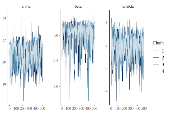
Not great, but it’ll do for now.

Extracting information from the posterior

Now we need to extract the posterior summaries of the parameters, as well as the diagnostics

# Extracting the summary statistics of the parameters
parameter_summary = fit$summary(c("alpha","beta","lambda"))
# Extractiing the diagnostics of the sampler
diagnoistics = data.frame(fit$diagnostic_summary())

In order to generalize this we could loop through different combinations of parameter values and then collect the summary and diagnostics for each pair of simulated parameter values. We do this below; where we use the code from the data simulation markdown to generate parameter values:

# keep the number of data points constant (could also vary this)
N = 100
#intercept
alpha = seq(0,20,length.out = 3)
#slope
beta = seq(1,10,length.out = 3)
#sigma
lambda = seq(0,0.3,length.out = 3)

#lastly we put it together in a dataframe called simulated_parameters
simulated_parameters = expand.grid(alpha = alpha,
                         beta = beta,
                         lambda = lambda,
                         N = N)

Now we write the loop that fits our model and collects diagnostics and summary statistics. Please note that we set refresh argument to 0 meaning that we omit most of the output from the sampling process, but have also set the chunk to results='hide' which means no output is generated

#Empty dataframe to collect estimates and diagnostics

results = data.frame()

#loop through the rows of the simulated parameters (i.e agents)
for(row in 1:nrow(simulated_parameters)){
  
  N = simulated_parameters$N[row]
  alpha = simulated_parameters$alpha[row]
  beta = simulated_parameters$beta[row]
  lambda = simulated_parameters$lambda[row]
  
  #given the simulated parameter values we generate binary responses (y's)
  x = seq(-20,40, length.out = N)
  # getting the probabilities from the model and the parameters
  p = lambda+(1-2*lambda)*(0.5+0.5*pracma::erf((x-alpha)/(sqrt(2)*beta)))
  # generating binary responses from the probabilities above
  y = rbinom(N,1,p)
  #fit model
  fit = model_obj2$sample(data = list(N =N, x = x, y =y),
                          seed = seeds,
                        #warm-up samples
                        iter_warmup = 500,
                        #inference samples
                        iter_sampling = 500,
                        #chains
                        chains = 4,
                        #parallel chains
                        parallel_chains = 4,
                        #refresh rate of printing
                        refresh = 0,
                        #adap delta argument default 0.9
                        adapt_delta = 0.9)
  #summary and diagnostics
  parameter_summary = fit$summary(c("alpha","beta","lambda"))
  diagnoistics = data.frame(fit$diagnostic_summary())
  
  #make a summary of the 4 chains  
  summary_diagnoistics = colMeans(diagnoistics)

  #combine all the information into a single dataframe: First diagnostics and then simulated values:
  parameter_summary = parameter_summary %>% 
    mutate(num_divergent = summary_diagnoistics[1],
           num_max_treedepth = summary_diagnoistics[2],
           ebfmi = summary_diagnoistics[3]) %>% 
    mutate(simulated_alpha = alpha,
           simulated_beta = beta,
           simulated_lambda = lambda,
           simulated_value = c(alpha,beta,lambda),
           trials = N)
  
  # bind the results to the results dataframe
  results = rbind(results, parameter_summary)
}

## Warning: 1 of 2000 (0.0%) transitions ended with a divergence.
## See https://mc-stan.org/misc/warnings for details.
## 
## Warning: 1 of 2000 (0.0%) transitions ended with a divergence.
## See https://mc-stan.org/misc/warnings for details.
## 
## Warning: 1 of 2000 (0.0%) transitions ended with a divergence.
## See https://mc-stan.org/misc/warnings for details.
## 
## Warning: 1 of 2000 (0.0%) transitions ended with a divergence.
## See https://mc-stan.org/misc/warnings for details.
## 
## Warning: 1 of 2000 (0.0%) transitions ended with a divergence.
## See https://mc-stan.org/misc/warnings for details.
## 
## Warning: 1 of 2000 (0.0%) transitions ended with a divergence.
## See https://mc-stan.org/misc/warnings for details.
## 
## Warning: 1 of 2000 (0.0%) transitions ended with a divergence.
## See https://mc-stan.org/misc/warnings for details.
## 
## Warning: 1 of 2000 (0.0%) transitions ended with a divergence.
## See https://mc-stan.org/misc/warnings for details.
## 
## Warning: 1 of 2000 (0.0%) transitions ended with a divergence.
## See https://mc-stan.org/misc/warnings for details.
## 
## Warning: 1 of 2000 (0.0%) transitions ended with a divergence.
## See https://mc-stan.org/misc/warnings for details.
## 
## Warning: 1 of 2000 (0.0%) transitions ended with a divergence.
## See https://mc-stan.org/misc/warnings for details.
## 
## Warning: 1 of 2000 (0.0%) transitions ended with a divergence.
## See https://mc-stan.org/misc/warnings for details.
## 
## Warning: 1 of 2000 (0.0%) transitions ended with a divergence.
## See https://mc-stan.org/misc/warnings for details.
## 
## Warning: 1 of 2000 (0.0%) transitions ended with a divergence.
## See https://mc-stan.org/misc/warnings for details.

Lets check the output.

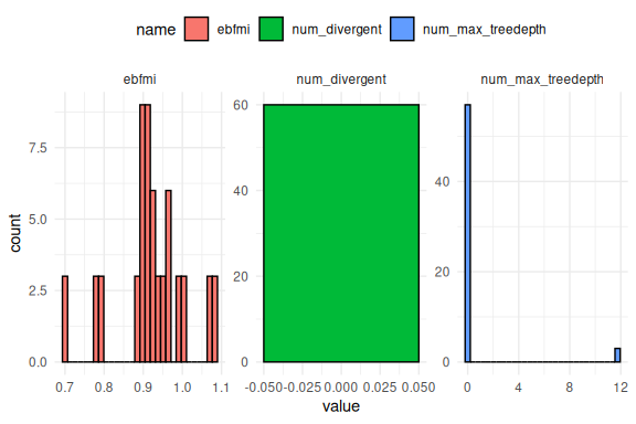
First how bad the sampling was across the simulations:

results %>% 
  select(num_divergent,num_max_treedepth,ebfmi) %>% 
  pivot_longer(everything()) %>% 
  ggplot(aes(x = value,fill = name))+
  geom_histogram(col = "black")+
  facet_wrap(~name, scales = "free")+
  theme_minimal()+
  theme(legend.position = "top")

## `stat_bin()` using `bins = 30`. Pick better value with `binwidth`.

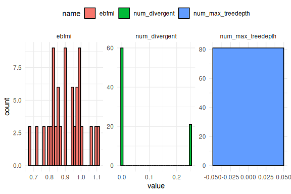
Is not to bad, but some of the simulations did have divergences.

Lets forget about that for now and plot the real parameter recovery i.e. simulated vs estimated parameter values.

results %>% 
  ggplot(aes(x = simulated_value, y = mean, ymin = q5, ymax = q95, fill = variable))+
  geom_pointrange(shape = 21, color = "black")+
  facet_wrap(~variable, scales = "free")+
  geom_abline()+
  theme_minimal()

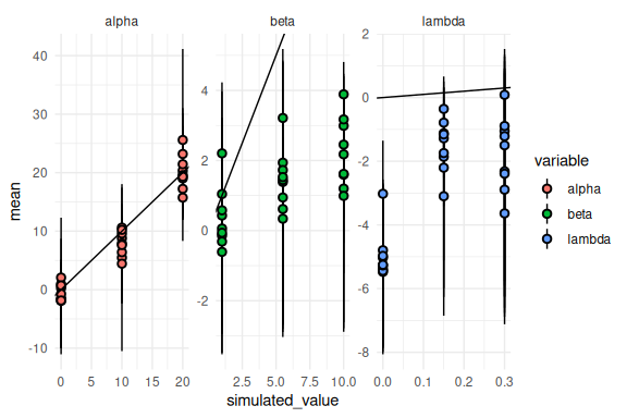
For all parameters, but alpha this looks terrible.

This is because the output from Stan is on the unconstrained scale (Note that the estimated y-axis for beta and lambda extends to negative values). If we transform them we get:

results %>% mutate(across(c(mean, q5, q95), 
                ~ ifelse(variable == "beta", exp(.),
                         ifelse(variable == "lambda", brms::inv_logit_scaled(.) / 2, .)))) %>% 
  ggplot(aes(x = simulated_value, y = mean, ymin = q5, ymax = q95, fill = variable))+
  geom_pointrange(shape = 21, color = "black")+
  facet_wrap(~variable, scales = "free")+
  geom_abline()+
  theme_minimal()

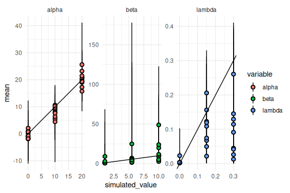
Much better!

Lets check the simulations that had a single divergent transition.

results %>% mutate(across(c(mean, q5, q95), 
                ~ ifelse(variable == "beta", exp(.),
                         ifelse(variable == "lambda", brms::inv_logit_scaled(.) / 2, .)))) %>% 
  mutate(divergent = ifelse(num_divergent > 0,T,F)) %>% 
  ggplot(aes(x = simulated_value, y = mean, ymin = q5, ymax = q95, fill = divergent))+
  geom_pointrange(shape = 21, color = "black")+
  facet_wrap(~variable, scales = "free")+
  geom_abline()+
  theme_minimal()

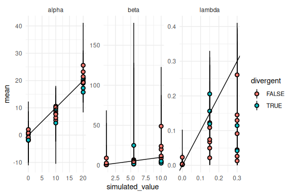
Not much of a pattern together with the fact that there weren’t that many divergent transisitions. Generally i would exclude all divergent transisitions for reporting parameter recovery.

As can be seen we have simulated discrete values, however one might want to do this continuously i.e. sampling parameter values from a distribution. I showcase this below together with a computationally more efficient way to conduct parameter recovery using parallelization.

Furrr and parallelization

First we get parameter values as before, now just with the parameters coming from a distribution.

Here I simulate parameter values from the same distribution we used for the prior for the model.

#number of simulations
N_sim = 20
# keep the number of data points constant (could also vary this)
N = 100
#intercept
alpha = rnorm(N_sim,20,10)
#slope
beta = exp(rnorm(N_sim,0,2))
#sigma
lambda = brms::inv_logit_scaled(rnorm(N_sim,-4,2) / 2)
#lastly we put it together in a dataframe called simulated_parameters

simulated_parameters = data.frame(alpha = alpha,
                                  beta = beta,
                                  lambda = lambda,
                                  N = N)

Now instead of looping through the rows, as before, we are going to use the power of furrr.

The furrr package allows us to send a list to a user specified function that then runs. The magic that furrr provides is that if given a list of lists furrr can distribute the jobs (i.e. the individual lists) across several “workers” (cpus of the computer). This means that instead of going through each of the rows of our dataframe above, we can evaluate them in parallel. How many rows can be run in parallel of cause depends on your compute power (the number of cpus in the computer).

The first step is to generate a list of lists from the dataframe, here we use the convenient wrapper function of “split”

# first we make a new colum that is just the row number
simulated_parameters$n_row = 1:nrow(simulated_parameters)

simulated_lists = split(simulated_parameters, simulated_parameters$n_row)

Next we initialize furrr by telling it how many cores / workers we want. You can check how many you have with the following code:

cores = parallelly::availableCores()
cores

## system 
##     64

Now given that each of our simulations already take 4 cores due to the parallelization of the chains, i would generally recommend not using more than the number of cores divided by 4. This entails that there are 4 cores for each iteration.

plan(multisession, workers = cores/4)

Next we need to define the function that is going to be run on the list.

This is essentially what we wrote inside the loop above.

Note that i also set adapt_delta to 0.99 to try and get rid of the last couple of divergences:

parameter_recovery = function(simulated_parameters){
   
  N = simulated_parameters$N
  alpha = simulated_parameters$alpha
  beta = simulated_parameters$beta
  lambda = simulated_parameters$lambda
  
  #given the simulated parameter values we generate binary responses (y's)
  x = seq(-20,40, length.out = N)
  # getting the probabilities from the model and the parameters
  p = lambda+(1-2*lambda)*(0.5+0.5*pracma::erf((x-alpha)/(sqrt(2)*beta)))
  # generating binary responses from the probabilities above
  y = rbinom(N,1,p)
  #fit model
  fit = model_obj2$sample(data = list(N =N, x = x, y =y),
                          seed = seeds,
                        #warm-up samples
                        iter_warmup = 500,
                        #inference samples
                        iter_sampling = 500,
                        #chains
                        chains = 4,
                        #parallel chains
                        parallel_chains = 4,
                        #refresh rate of printing
                        refresh = 0,
                        #adap delta argument default 0.9
                        adapt_delta = 0.99)
  #summary and diagnostics
  parameter_summary = fit$summary(c("alpha","beta","lambda"))
  diagnoistics = data.frame(fit$diagnostic_summary())
  
  #make a summary of the 4 chains  
  summary_diagnoistics = colMeans(diagnoistics)

  #combine all the information into a single dataframe: First diagnositcs and then simulated values:
  parameter_summary = parameter_summary %>% 
    mutate(num_divergent = summary_diagnoistics[1],
           num_max_treedepth = summary_diagnoistics[2],
           ebfmi = summary_diagnoistics[3]) %>% 
    mutate(simulated_alpha = alpha,
           simulated_beta = beta,
           simulated_lambda = lambda,
           simulated_value = c(alpha,beta,lambda),
           trials = N)
  
  return(parameter_summary)
}

We can check that it works, by giving the function the first list of our lists of lists:

parameter_recovery(simulated_lists[[1]])

## Running MCMC with 4 parallel chains...
## 
## Chain 2 finished in 0.3 seconds.
## Chain 3 finished in 0.4 seconds.
## Chain 4 finished in 0.4 seconds.
## Chain 1 finished in 0.7 seconds.
## 
## All 4 chains finished successfully.
## Mean chain execution time: 0.4 seconds.
## Total execution time: 0.9 seconds.

## # A tibble: 3 × 18
##   variable  mean median    sd   mad      q5    q95  rhat ess_bulk ess_tail
##   <chr>    <dbl>  <dbl> <dbl> <dbl>   <dbl>  <dbl> <dbl>    <dbl>    <dbl>
## 1 alpha    -8.24  -8.44  3.98 3.73  -14.4   -1.65   1.01     554.     402.
## 2 beta      2.30   2.80  1.27 0.683  -0.543  3.46   1.02     352.     335.
## 3 lambda   -2.85  -2.16  2.08 2.00   -6.83  -0.518  1.02     407.     796.
## # ℹ 8 more variables: num_divergent <dbl>, num_max_treedepth <dbl>,
## #   ebfmi <dbl>, simulated_alpha <dbl>, simulated_beta <dbl>,
## #   simulated_lambda <dbl>, simulated_value <dbl>, trials <dbl>

Works wonders!

Now we do the last setup of furrr. Inorder to handle if any errors occur we can use the convenient “possibly” function. Here we put in our function and tells it what to do if it runs into an error. Here we specify that it returns “Error” if it runs into an error.

fit_parameter_recovery = possibly(.f = parameter_recovery, otherwise = "Error")

Double checking that the function works:

test = fit_parameter_recovery(simulated_lists[[1]])

## Running MCMC with 4 parallel chains...
## 
## Chain 1 finished in 0.2 seconds.
## Chain 3 finished in 0.1 seconds.
## Chain 2 finished in 0.2 seconds.
## Chain 4 finished in 0.2 seconds.
## 
## All 4 chains finished successfully.
## Mean chain execution time: 0.2 seconds.
## Total execution time: 0.4 seconds.

Lastly, we run furrr with the following code. Note the .progress = T argument gives you a progess bar, if you have more than one worker running.

results <- future_map(simulated_lists,
                      ~fit_parameter_recovery(.x),
                      .options = furrr_options(seed = TRUE),
                      .progress = T)

## Warning: 47 of 2000 (2.0%) transitions hit the maximum treedepth limit of 10.
## See https://mc-stan.org/misc/warnings for details.
## 
## Warning: 47 of 2000 (2.0%) transitions hit the maximum treedepth limit of 10.
## See https://mc-stan.org/misc/warnings for details.

Now the results are going to be in lists just as the input was, but we can quickly make it a dataframe

results = map_dfr(results, bind_rows)

Checking the output:

Diagnostics

results %>% 
  select(num_divergent,num_max_treedepth,ebfmi) %>% 
  pivot_longer(everything()) %>% 
  ggplot(aes(x = value,fill = name))+
  geom_histogram(col = "black")+
  facet_wrap(~name, scales = "free")+
  theme_minimal()+
  theme(legend.position = "top")

## `stat_bin()` using `bins = 30`. Pick better value with `binwidth`.

Is not to bad, but now we have a simulation that hit max_treedepth. We forget about that for now and plot the parameter recovery plot again i.e. simulated vs estimated parameter values.

Again remembering the transformations

results %>% mutate(across(c(mean, q5, q95), 
                ~ ifelse(variable == "beta", exp(.),
                         ifelse(variable == "lambda", brms::inv_logit_scaled(.) / 2, .)))) %>% 
  ggplot(aes(x = simulated_value, y = mean, ymin = q5, ymax = q95, fill = variable))+
  geom_pointrange(shape = 21, color = "black")+
  facet_wrap(~variable, scales = "free")+
  geom_abline()+
  theme_minimal()

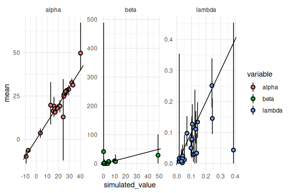
Not too bad! Lets see which of which of the simulations had tree depth issues: transitions.

results %>% mutate(across(c(mean, q5, q95), 
                ~ ifelse(variable == "beta", exp(.),
                         ifelse(variable == "lambda", brms::inv_logit_scaled(.) / 2, .)))) %>% 
  mutate(tree_depth = ifelse(num_max_treedepth > 0,T,F)) %>% 
  ggplot(aes(x = simulated_value, y = mean, ymin = q5, ymax = q95, fill = tree_depth))+
  geom_pointrange(shape = 21, color = "black")+
  facet_wrap(~variable, scales = "free")+
  geom_abline()+
  theme_minimal()

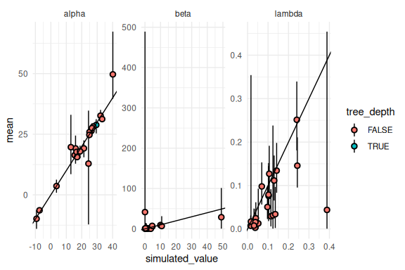
Not much to see. One could increase the max_treedepth argument and get good sampling across the board, this is left to the reader.

Final remarks

This finishes the section on parameter recovery. Here we showcase one of the first main tools to ensure that everything works as it should. Parameter recovery is slowly becoming more standard in the computational cognitive science literature with custom made models, which is great as you will not find many papers before 2015-2018, reporting parameter recovery. However, as with many things the methodological field has already moved quite a bit beyond one of the main contributors to including parameter recovery i.e. ten simple rules of computational modeling. This is the topic for the next markdown 6.y simulation based calibration (SBC). In SBC we want to ensure that the estimated parameter value contains the simulated parameter value to the extent of the credibility intervals. Thus with a 95 % credibility interval as above, we want to make sure that the simulated value is within this interval in 95% of cases, not more and not less.

SBC references

Share on

X (formerly Twitter) Facebook LinkedIn

Jesper Fischer Ehmsen