Building Multivariate Models

16 minute read

Published: February 05, 2025

Multivariate Copula Modeling

This R markdown is for showcasing how one can use copulas to build cogntive computational multivariate models and what can be gained from it. With an example of decision making with confidence ratings.

Table of content

Overview
Signal detection theory
Linking SDT to response times and confidence ratings
Likelihood functions
Simulations
Combing the marginals with a copula
Further exploration

Packages and setup

packages = c("brms","tidyverse","bayesplot",
             "pracma","here", "patchwork",
             "posterior","HDInterval","ordbetareg",
             "loo", "furrr","cmdstanr","mnormt","Rlab")


do.call(pacman::p_load, as.list(packages))

knitr::opts_chunk$set(echo = TRUE)

register_knitr_engine(override = FALSE)

set.seed(123)

Overview.

Now that we have seen that we can build and implement flexible multivariate models using copulas where the marginal distributions are conditional and the marginals can be discrete. We now move to the fun part of using this in practice and building multivariate models. To motivate this we will investigate perceptual decision making task where subjects view a set of random dots move. Most of these dots move randomly, but a certainty procentage (coherence) move left or right. Subjects are then to make a binary decision of whether the majority of dots moved left or right (the type 1 decision) and then make a confidence judgement on a VAS-rating scale from Guessing to completely certain. Additional to collecting binary choices and confidence ratings we will also collect response times to the type 1 decision. This means we have 3 main measures of our experiment and 1 experimentally manipulated variable. Inorder to build a joint model of these 3 response variable and their relationship with the stimulus intensity (coherence) we will start with a known theory of the type 1 decision, namely the signal detection framework / theory (SDT)

Signal detection theory.

From a signal detection perspective the task can be described from the observer by assuming that there is an internal decision variable x that is noisy representation of the stimulus coherence c. This can be written x ∼ 𝒩(c, σ)

where σ is internal noise in the observer. When the observer then have to make a binary decision of whether the stimulus was moving left or right we assume that they compare x to a criterion α such that the subject responds “right” if x > α and otherwise respond “left”. We can easily calculate the probability that x is greater than α this is done throught the cummulative normal distribution function Φ(.) which gives us the probability of x being equal to or less than a particular value i.e. α. Thus

\[P("Right" | c, \sigma) = P(x > \alpha | c, \sigma)\]

Using that the probability that x > α must be equal to the probability that x ≤ α

$= 1-P(x \le \alpha | c, \sigma) = 1 - \Phi\left(\frac{\alpha-c}{\sigma}\right)$ And then using the symmetric of the cummulative gaussian we can go back i.e.

\[1 - \Phi\left(\frac{\alpha-c}{\sigma}\right) = \Phi\left(\frac{c-\alpha}{\sigma}\right)\]

This function describes how the probability of choosing “right” increases as the coherence. In this formulation, the threshold parameter α defines the point of subjective equality (where the observer is equally likely to choose left or right), and the slope of the function is governed by the noise parameter σ. Smaller values of σ indicating a steeper (more precise) psychometric function.

To accommodate potential lapses or guessing behavior, the psychometric function is often extended with lower and upper asymptotes: $P("Right" | c) = \gamma + (1 - \gamma - \lambda) \cdot \Phi\left(\frac{c-\alpha}{\sigma}\right)$

This formulation is more flexible than the standard SDT fomulation where we start with two different stimuli (sometimes the second stimulus is no stimulus i.e. x₁ ∼ 𝒩(0, σ)) that are internally represented as before i.e. x₁ ∼ 𝒩(μ₁, σ) , x₂ ∼ 𝒩(μ₂, σ). Now d′ is the difference in means between the two distributions expressed in their shared standard deviation i.e. $d’ = \frac{\mu_2 - \mu_1}{\sigma}$. The Decision crition is then:

Linking SDT to response times and confidence ratings

Now that we have a theoretically informed “computational” model of how subjects decide whether they are going to respond “left” or “right” based on the coherence level we can link this to the response times (RT) and the confidence ratings (Conf). There are infinity many ways of how this can be done, but below i’m going to argue for a particular way that is both intuative and has been used in the litterature before. First im going to decribe is intuatively and then integrate it with the decision making litterature at last.

When making a Binary decision of whether the dots are moving leftwards or rightwards its intuative that the more dots are moving in either direction will make the task easier and thus one would expect that a subject would respond more consistently as the coherence increased. This rationale is essentially what is baked into the psychometric function. However how hard a particular trial (that is a particular coherence level) will depend on the threshold α and sensitivity $\frac{1}{\beta}$ of that individual. A subject with no bias (i.e. α = 0) and a steep slope will have a very easy time with high coherence levels, whereas a subject with less steep slopes will find them more ambiguous.

One way to quantify this dificulty in each trial is to compute the uncertainty of the choice probability predicted by SDT. Several such uncertainties exisits and have been used previously in the litterature, but here we use the entropy formally defined as.

$H(X) = - \sum_{i=1}^{n} p(x_i) \\ \log p(x_i)$ which simplifies greatly with two choices (i.e. the probability of responding “Right”, is also just the complement probability of responding left).

H(X) = −(p(x_i) ⋅ log p(x_i) + (1 − p(x_i) ⋅ log (1 − p(x_i)) Where p(x_i) we will define as the probability of responding “Right”.

Previous litterature just following Shannon’s information theoretical contribution, which included the scientists Hick and Hymann showed that as the entropy of a decision increases so does the response time in a linear manner to the entropy i.e.

R**T ∝ H(X) Intuatively, this makes sense. If you have to make a decision based on limited evidence (i.e. its close to the transistion point of where you would respond one or the other) you will be slower, whereas a decision made where you are sure of which direction the dots moved, you would also respond quickly.

The same rationale holds for confidence ratings but here as decision uncertainty H(X) increases Confidence decreases Con**f ∝ −H(X)

lastly we might think that the subject has access to some metacognitive ability, i.e. they have an idea of whether they were correct or incorrect in the type-1 decision (“Right” or “Left”). If this is the case then firstly the confidence ratings would be quite different between correct and incorrect choices but this difference would also be modulated by the dificulty of the trial. Imagine a very easy trial were you end up making a misstake and thus responds “Left” eventhough 90% of the dots moved “Right”. When giving the confidence ratings here you will be sure that you were incorrect whereas in the scinario where you responded correctly you will be sure you made the right choice. When the dificulty then increases the confidence in the correct decision will decrease whereas the confidence in the incorrect decision might increases, reflecting greater uncertainty and doubt in whether you were correct. These increase and decreases should then peak when decision uncertainty is maximal which happens around the decision threshold α whereafter the task will become easier again (just in the other direction, such that the dots are moving more to the left).

Likelihood functions

In order to map the observed measures into a statistical model we need a marginal distribution for each of the observed measures. In this step of the model building procedure its important to comply with the natural bounds of the outcome measures, i.e. not using a normal distribution to model bounded data or discrete data. The natural choice for the binary decision data is the bernoulli distribution, whereas for response time we will use a shifted lognormal distribution and for the COnfidence-ratings (that are bounded between 0 and 1), we will use the ordered beta distribution. The marginal distribution for these are shown below:

where Y_choice ∈ {0, 1} (e.g. 1 = Right), Φ(⋅) is the standard normal CDF, α the criterion, and σ the SD of internal noise. Support: p(c) ∈ (0, 1).

$Y_{\text{choice}} \\\sim\\ \mathrm{Bernoulli}\big( p(c) \big), \\ P("Right" | c) = \gamma + (1 - \gamma - \lambda) \cdot \Phi\left(\frac{c-\alpha}{\sigma}\right)$ (R**T + τ) ∼ LogNormal(μ_R**T, σ_R**T), where RT is the observed RT (seconds), τ is a shift / non-decision time.

\[Y_{\text{conf}} \\\sim\\ \begin{cases} c_0, & \text{if } Y_{\text{conf}} = 0, \\ (1 - c_0 - c_1)\\ \mathrm{Beta}\\\big(\mu_C,\\\phi_C\big), & \text{if } 0 < Y_{\text{conf}} < 1, \\ c_1, & \text{if } Y_{\text{conf}} = 1, \end{cases}\]

With Beta(.) being the beta-distribution parameterized with mean and precision.

Simulations

Now before joining these marginally conditional statistical models with copulas I’ll below simulate data from this model to display what is assumed for different parameter values.

setting parameter values

alpha = c(-10,0,10)
alpha = 0
beta = exp(c(1,3))
beta = 2
lapse = brms::inv_logit_scaled(c(-4,-3,-2))
lapse = brms::inv_logit_scaled(c(-4))

rt_int = c(-2,-1)
rt_slope = c(1,2)
rt_sd = exp(c(-1))
rt_ndt = c(0.1)


conf_int = c(-2,-1)
conf_slope = c(0.5,1)
conf_ACC = c(1,2)
conf_slope_ACC = c(-2,-4)
conf_prec = exp(c(4))
c0 = brms::logit_scaled(c(0.01))
c1 = brms::logit_scaled(c(0.1)) + exp(c(2))

source(here::here("Analysis","Scripts","Utility.r"))

get_trial_data = function(df){
  
  set.seed(123)

  x = seq(-20,20,by = 0.1)  
  p = psychometric(x,df[1,])
  bin = rbinom(length(p),1,p)
  ACC = ifelse(x > 0 & bin == 1, 1, ifelse(x < 0 & bin == 0,1,0))
  rt_mu = RT_mean(p,df[1,])
  conf_mu = conf_mean(p,ACC,df[1,])
  
  
  rts = rlnorm(length(rt_mu),rt_mu, df$rt_sd) + df$rt_ndt
  conf = rordbeta(length(conf_mu),
                  brms::inv_logit_scaled(conf_mu),
                  df$conf_prec,
                  cutpoints = c(df$c0,df$c1))
  
  data.frame(x = x, p = p, bin = bin, ACC = ACC, rt_mu = rt_mu, conf_mu = conf_mu, rts = rts, conf = conf)
}



param_grid <- expand.grid(
  alpha = alpha,
  beta = beta,
  lapse = lapse,
  rt_int = rt_int,
  rt_slope = rt_slope,
  rt_sd = rt_sd,
  rt_ndt = rt_ndt,
  conf_int = conf_int,
  conf_slope = conf_slope,
  conf_ACC = conf_ACC,
  conf_slope_ACC = conf_slope_ACC,
  conf_prec = conf_prec,
  c0 = c0,
  c1 = c1,
  KEEP.OUT.ATTRS = FALSE,
  stringsAsFactors = FALSE
)

dfs = param_grid %>% 
  rowwise() %>% 
  mutate(resps = list(get_trial_data(cur_data())),
         draw = 1:n()) %>% ungroup()


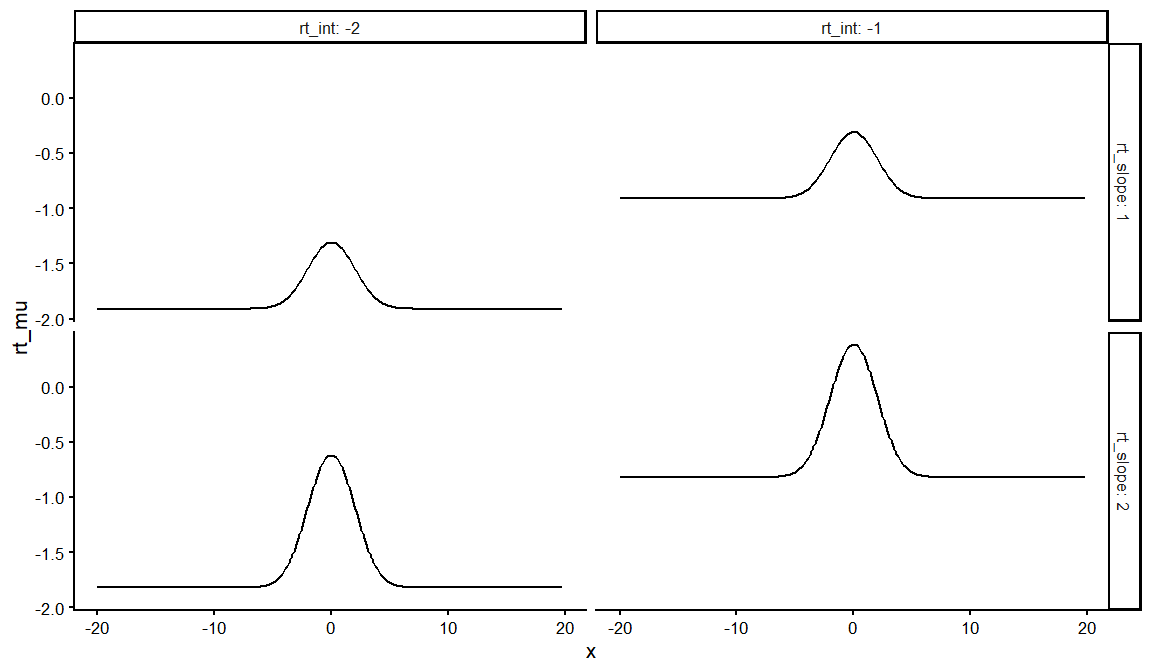
dfs  %>% 
  distinct(rt_int, rt_slope, rt_ndt, draw, .keep_all = TRUE) %>% 
  unnest(resps)%>% filter(ACC == 1) %>% 
  ggplot(aes(x = x, y = rt_mu))+
  geom_line()+
  facet_grid(rt_slope~rt_int, labeller = label_both)+
  theme_classic(base_size = 16)

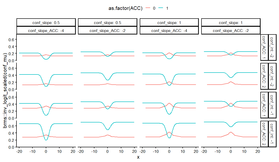
dfs  %>% 
  distinct(conf_int, conf_slope, conf_ACC, conf_slope_ACC, draw, .keep_all = TRUE) %>% 
  unnest(resps) %>% 
  ggplot(aes(x = x, y = brms::inv_logit_scaled(conf_mu), col = as.factor(ACC)))+
  geom_line()+
  facet_grid(conf_int+conf_ACC~conf_slope+ conf_slope_ACC, labeller = label_both)+
  theme_classic(base_size = 16)+
  theme(legend.position = "top")

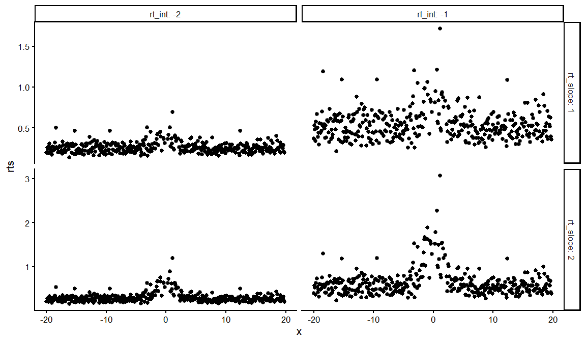
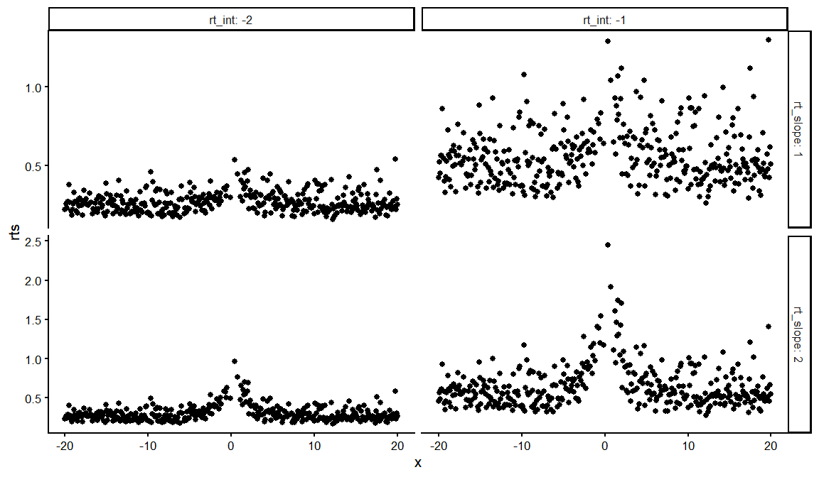
dfs  %>% 
  distinct(rt_int, rt_slope, rt_ndt, draw, .keep_all = TRUE) %>% 
  unnest(resps)%>% filter(ACC == 1) %>% 
  ggplot(aes(x = x, y = rts))+
  geom_point()+
  facet_grid(rt_slope~rt_int, labeller = label_both, scales = "free_y")+
  theme_classic(base_size = 16)

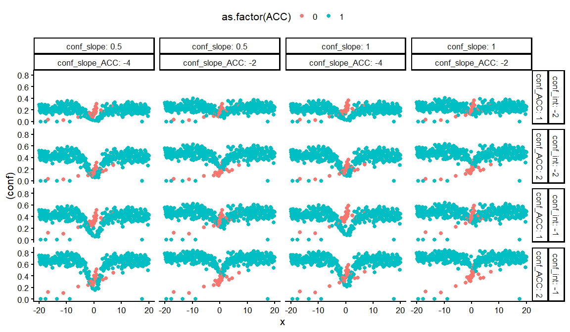
dfs  %>% 
  distinct(conf_int, conf_slope, conf_ACC, conf_slope_ACC, draw, .keep_all = TRUE) %>% 
  unnest(resps) %>% 
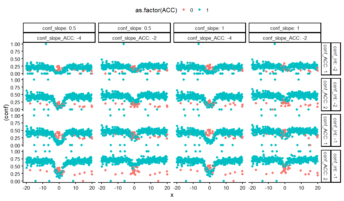
  ggplot(aes(x = x, y = (conf), col = as.factor(ACC)))+
  geom_point()+
  facet_grid(conf_int+conf_ACC~conf_slope+ conf_slope_ACC, labeller = label_both)+
  theme_classic(base_size = 16)+
  theme(legend.position = "top")

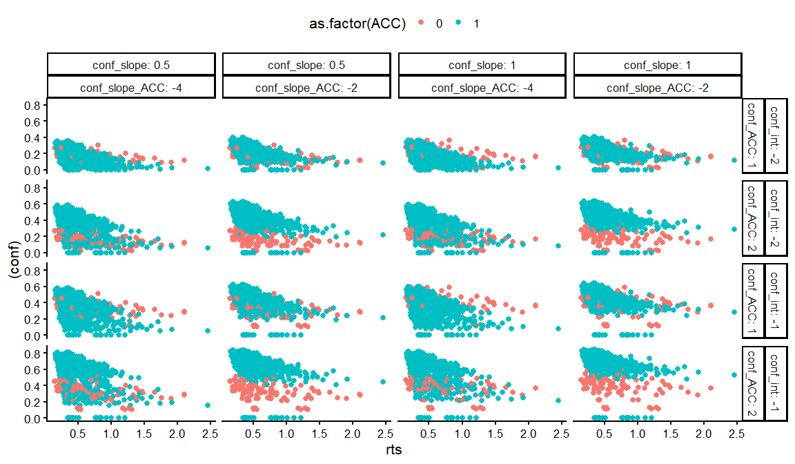
dfs  %>% 
  distinct(conf_int, conf_slope, conf_ACC, conf_slope_ACC,rt_int, rt_slope, rt_ndt, draw, .keep_all = TRUE) %>% 
  unnest(resps) %>% 
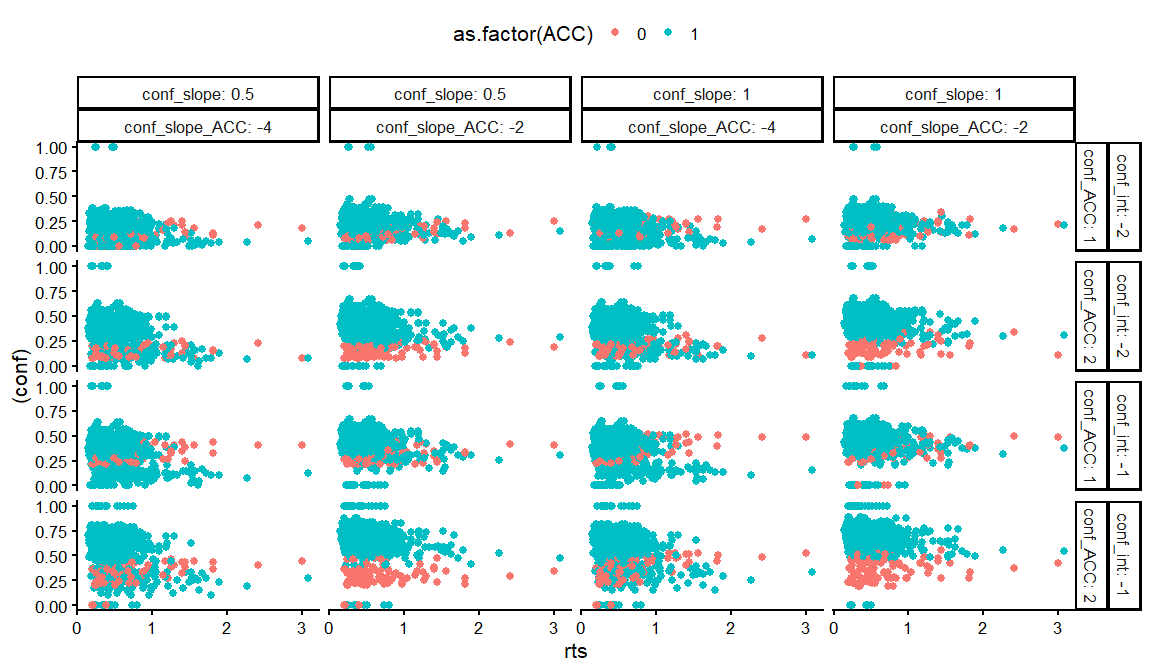
  ggplot(aes(x = rts, y = (conf), col = as.factor(ACC)))+
  geom_point()+
  facet_grid(conf_int+conf_ACC~conf_slope+ conf_slope_ACC, labeller = label_both)+
  theme_classic(base_size = 16)+
  theme(legend.position = "top")

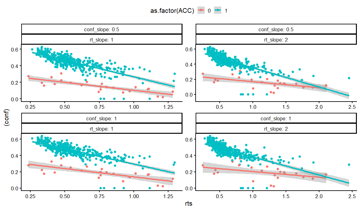
dfs  %>% 
  distinct(conf_int, conf_slope, conf_ACC, conf_slope_ACC,rt_int, rt_slope, rt_ndt, draw, .keep_all = TRUE) %>% 
  unnest(resps) %>% 
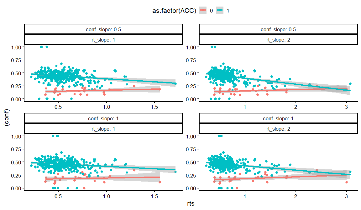
  filter(rt_int == -1,conf_ACC == 2, conf_int == -2) %>% 
  filter(conf_slope_ACC == -2) %>% 
  ggplot(aes(x = rts, y = (conf), col = as.factor(ACC)))+
  geom_point()+
  geom_smooth(method = "lm")+
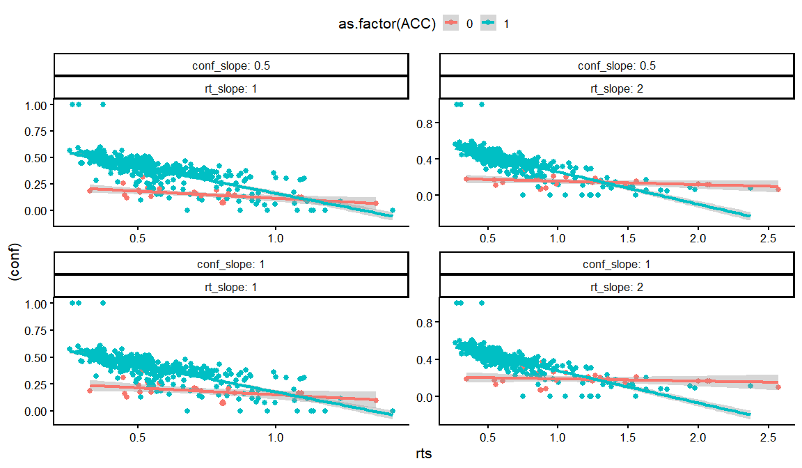
  facet_wrap(conf_slope~rt_slope, labeller = label_both, scales = "free")+
  theme_classic(base_size = 16)+
  theme(legend.position = "top")

## `geom_smooth()` using formula = 'y ~ x'

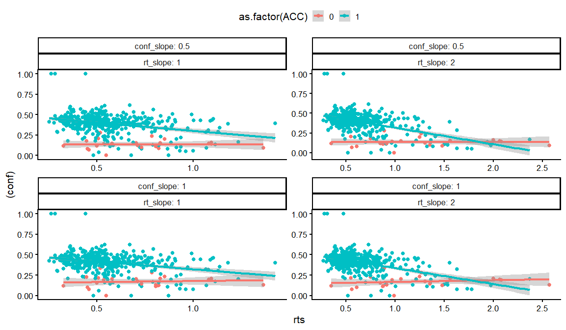
dfs  %>% 
  distinct(conf_int, conf_slope, conf_ACC, conf_slope_ACC,rt_int, rt_slope, rt_ndt, draw, .keep_all = TRUE) %>% 
  unnest(resps) %>% 
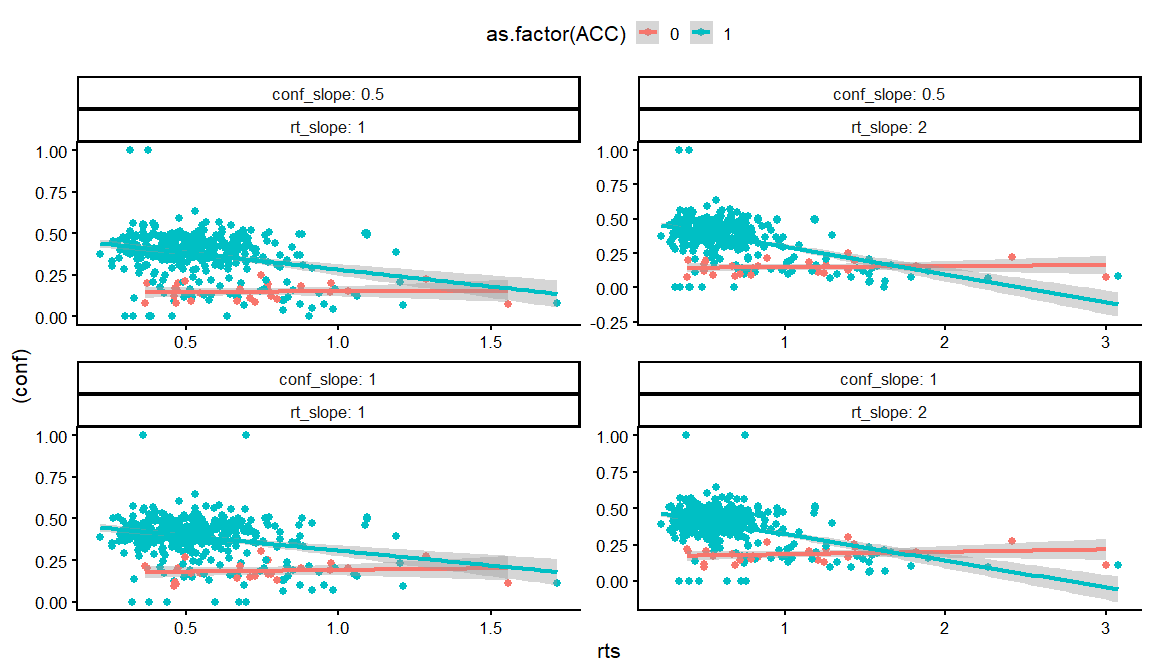
  filter(rt_int == -1,conf_ACC == 2, conf_int == -2) %>% 
  filter(conf_slope_ACC == -4) %>% 
  ggplot(aes(x = rts, y = (conf), col = as.factor(ACC)))+
  geom_point()+
  geom_smooth(method = "lm")+
  facet_wrap(conf_slope~rt_slope, labeller = label_both, scales = "free")+
  theme_classic(base_size = 16)+
  theme(legend.position = "top")

## `geom_smooth()` using formula = 'y ~ x'

Combing the marginals with a copula

Now as we saw in the previous markdowns, we can glue these conditially dependent statistical models together using copulas.

param_grid <- expand.grid(
  alpha = alpha,
  beta = beta,
  lapse = lapse,
  rt_int = rt_int,
  rt_slope = rt_slope,
  rt_sd = rt_sd,
  rt_ndt = rt_ndt,
  conf_int = conf_int,
  conf_slope = conf_slope,
  conf_ACC = conf_ACC,
  conf_slope_ACC = conf_slope_ACC,
  conf_prec = conf_prec,
  c0 = c0,
  c1 = c1,
  rho12 = c(-0.8,0,0.8),
  rho13 = c(-0.8,0,0.8),
  rho23 = c(-0.8,0,0.8),
  KEEP.OUT.ATTRS = FALSE,
  stringsAsFactors = FALSE
) %>%
  rowwise() %>%
  filter(is_pos_def(rho12, rho13, rho23)) %>%
  ungroup()



get_trial_data_copula = function(df){

  set.seed(123)

  x = seq(-20,20,by = 0.1)  
  p = psychometric(x,df[1,])
  rt_mu = RT_mean(p,df[1,])

  us = get_copula_vec(df, length(x))  

  bin = qbinom(us$u_bin,1,p)
  ACC = ifelse(x > 0 & bin == 1, 1, ifelse(x < 0 & bin == 0,1,0))
  conf_mu = conf_mean(p,ACC,df[1,])

  
  rts = qlnorm(us$u_rt,rt_mu, df$rt_sd) + df$rt_ndt
  
  conf = qordbeta(us$u_vas,
                  brms::inv_logit_scaled(conf_mu),
                  df$conf_prec,
                  df$c0,
                  df$c1)
  
  
  data.frame(x = x, p = p, bin = bin, ACC = ACC, rt_mu = rt_mu, conf_mu = conf_mu, rts = rts, conf = conf)
}

dfs = param_grid %>% 
  rowwise() %>% 
  mutate(resps = list(get_trial_data_copula(cur_data())),
         draw = 1:n()) %>% ungroup()



dfs  %>% 
  distinct(rt_int, rt_slope, rt_ndt, draw, .keep_all = TRUE) %>% 
  unnest(resps)%>% 
  filter(ACC == 1) %>% 
  ggplot(aes(x = x, y = rts))+
  geom_point()+
  facet_grid(rt_slope~rt_int, labeller = label_both, scales = "free_y")+
  theme_classic(base_size = 16)

dfs  %>% 
  distinct(conf_int, conf_slope, conf_ACC, conf_slope_ACC, draw, .keep_all = TRUE) %>% 
  unnest(resps) %>% 
  ggplot(aes(x = x, y = (conf), col = as.factor(ACC)))+
  geom_point()+
  facet_grid(conf_int+conf_ACC~conf_slope+ conf_slope_ACC, labeller = label_both)+
  theme_classic(base_size = 16)+
  theme(legend.position = "top")

dfs  %>% 
  distinct(conf_int, conf_slope, conf_ACC, conf_slope_ACC,rt_int, rt_slope, rt_ndt, draw, .keep_all = TRUE) %>% 
  unnest(resps) %>% 
  ggplot(aes(x = rts, y = (conf), col = as.factor(ACC)))+
  geom_point()+
  facet_grid(conf_int+conf_ACC~conf_slope+ conf_slope_ACC, labeller = label_both)+
  theme_classic(base_size = 16)+
  theme(legend.position = "top")

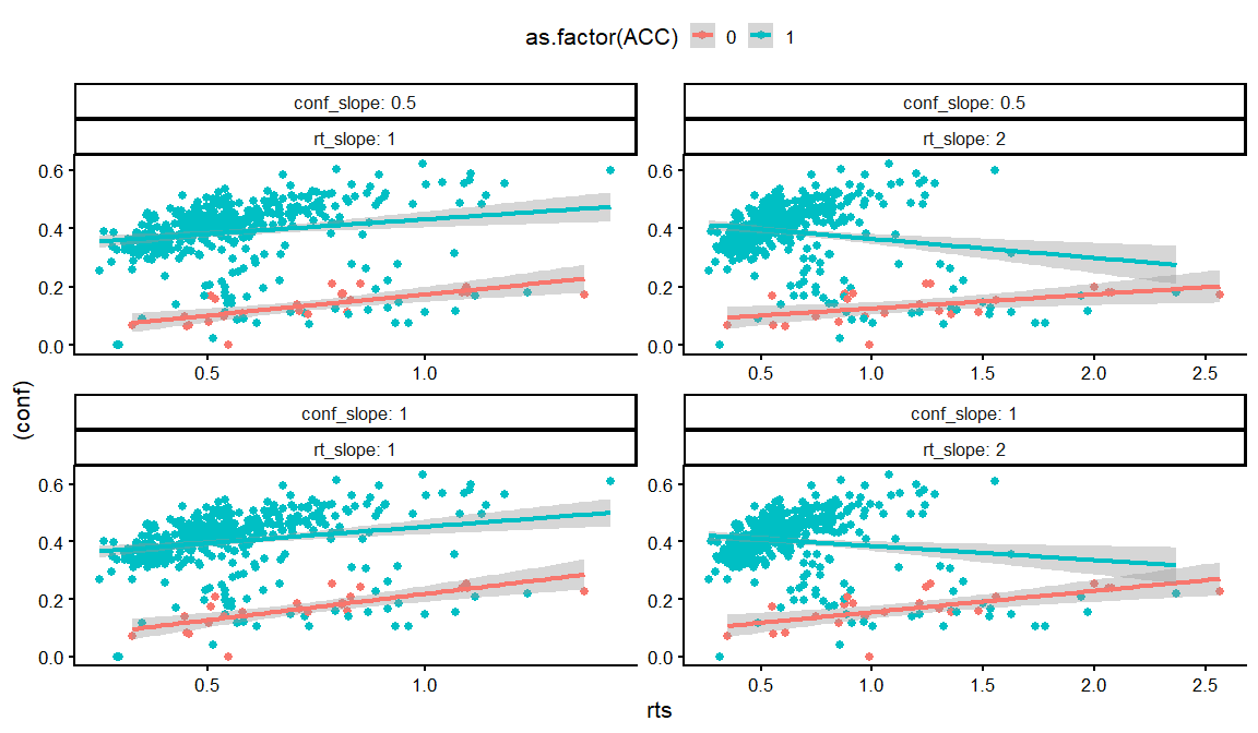
dfs  %>% 
  distinct(conf_int, conf_slope, conf_ACC, conf_slope_ACC,rt_int, rt_slope, rt_ndt, draw, .keep_all = TRUE) %>% 
  unnest(resps) %>% 
  filter(rt_int == -1,conf_ACC == 2, conf_int == -2) %>% 
  filter(conf_slope_ACC == -2) %>% 
  ggplot(aes(x = rts, y = (conf), col = as.factor(ACC)))+
  geom_point()+
  geom_smooth(method = "lm")+
  facet_wrap(conf_slope~rt_slope, labeller = label_both, scales = "free")+
  theme_classic(base_size = 16)+
  theme(legend.position = "top")

## `geom_smooth()` using formula = 'y ~ x'

dfs  %>% filter(rho12 == 0, rho13 == 0, rho23 == -0.8) %>% 
  distinct(conf_int, conf_slope, conf_ACC, conf_slope_ACC,rt_int, rt_slope, rt_ndt, draw, .keep_all = TRUE) %>% 
  unnest(resps) %>% 
  filter(rt_int == -1,conf_ACC == 2, conf_int == -2) %>% 
  filter(conf_slope_ACC == -4) %>% 
  ggplot(aes(x = rts, y = (conf), col = as.factor(ACC)))+
  geom_point()+
  geom_smooth(method = "lm")+
  facet_wrap(conf_slope~rt_slope, labeller = label_both, scales = "free")+
  theme_classic(base_size = 16)+
  theme(legend.position = "top")

## `geom_smooth()` using formula = 'y ~ x'

dfs  %>% filter(rho12 == 0, rho13 == 0, rho23 == -0.8) %>% 
  distinct(conf_int, conf_slope, conf_ACC, conf_slope_ACC,rt_int, rt_slope, rt_ndt, draw, .keep_all = TRUE) %>% 
  unnest(resps) %>% 
  filter(rt_int == -1,conf_ACC == 2, conf_int == -2) %>% 
  filter(conf_slope_ACC == -4) %>% 
  ggplot(aes(x = rts, y = (conf), col = as.factor(ACC)))+
  geom_point()+
  geom_smooth(method = "lm")+
  facet_wrap(conf_slope~rt_slope, labeller = label_both, scales = "free")+
  theme_classic(base_size = 16)+
  theme(legend.position = "top")

## `geom_smooth()` using formula = 'y ~ x'

dfs  %>% filter(rho12 == 0, rho13 == 0, rho23 == 0) %>% 
  distinct(conf_int, conf_slope, conf_ACC, conf_slope_ACC,rt_int, rt_slope, rt_ndt, draw, .keep_all = TRUE) %>% 
  unnest(resps) %>% 
  filter(rt_int == -1,conf_ACC == 2, conf_int == -2) %>% 
  filter(conf_slope_ACC == -4) %>% 
  ggplot(aes(x = rts, y = (conf), col = as.factor(ACC)))+
  geom_point()+
  geom_smooth(method = "lm")+
  facet_wrap(conf_slope~rt_slope, labeller = label_both, scales = "free")+
  theme_classic(base_size = 16)+
  theme(legend.position = "top")

## `geom_smooth()` using formula = 'y ~ x'

dfs  %>% filter(rho12 == 0, rho13 == 0, rho23 == 0.8) %>% 
  distinct(conf_int, conf_slope, conf_ACC, conf_slope_ACC,rt_int, rt_slope, rt_ndt, draw, .keep_all = TRUE) %>% 
  unnest(resps) %>% 
  filter(rt_int == -1,conf_ACC == 2, conf_int == -2) %>% 
  filter(conf_slope_ACC == -4) %>% 
  ggplot(aes(x = rts, y = (conf), col = as.factor(ACC)))+
  geom_point()+
  geom_smooth(method = "lm")+
  facet_wrap(conf_slope~rt_slope, labeller = label_both, scales = "free")+
  theme_classic(base_size = 16)+
  theme(legend.position = "top")

## `geom_smooth()` using formula = 'y ~ x'

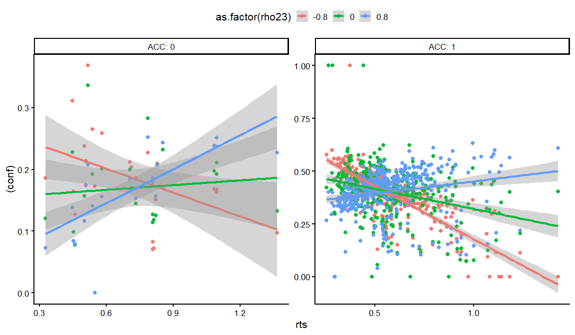
dfs  %>% filter(rho12 == 0, rho13 == 0) %>% 
  distinct(rho23,conf_int, conf_slope, conf_ACC, conf_slope_ACC,rt_int, rt_slope, rt_ndt, draw, .keep_all = TRUE) %>% 
  unnest(resps) %>% 
  filter(rt_int == -1,conf_ACC == 2, conf_int == -2,conf_slope == 1, rt_slope == 1) %>% 
  filter(conf_slope_ACC == -4) %>% 
  ggplot(aes(x = rts, y = (conf), col = as.factor(rho23)))+
  geom_point()+
  geom_smooth(method = "lm")+
  facet_wrap(~ACC, labeller = label_both, scales = "free")+
  theme_classic(base_size = 16)+
  theme(legend.position = "top")

## `geom_smooth()` using formula = 'y ~ x'

Further exploration

Share on

X (formerly Twitter) Facebook LinkedIn

Jesper Fischer Ehmsen