
Continous Copulas
Published:
- Multivariate Copula Modeling
This R markdown is for Showcasing the continous gaussian copula in non-gaussian marginals.
Table of content
Packages and setup
packages = c("brms","tidyverse","bayesplot",
             "pracma","here", "patchwork",
             "posterior","HDInterval",
             "loo", "furrr","cmdstanr","mnormt")


do.call(pacman::p_load, as.list(packages))

knitr::opts_chunk$set(echo = TRUE)

register_knitr_engine(override = FALSE)

set.seed(123)
Overview.
In this markdown the goal is to build on the previous markdown showcasing the trivial copula implementation of a gaussian copulas with two gaussian maginals. Here I want to extend that markdown into a gaussian copula with non-gaussian maginals.
Non Gaussian Marginals
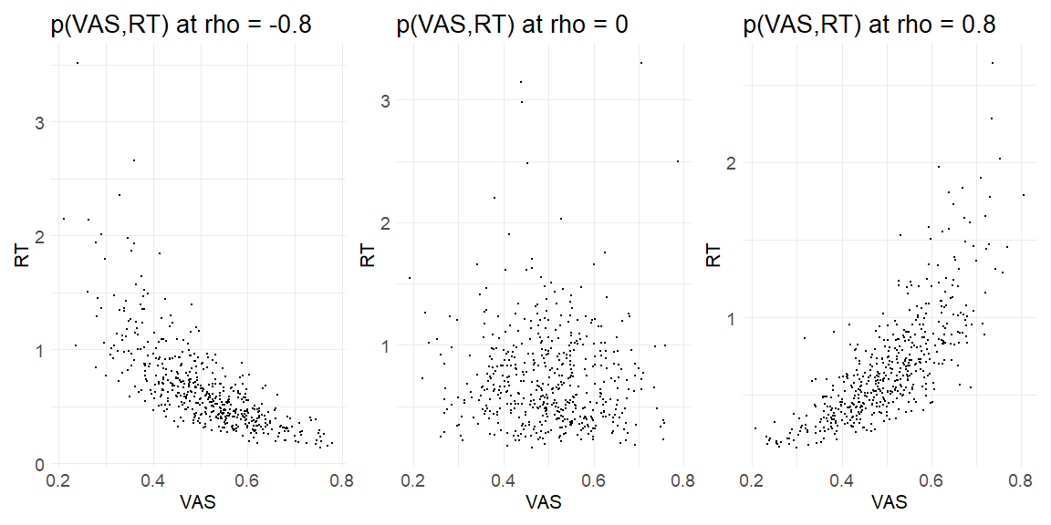
Lets say we observe some VAS-ratings (VAS) bounded between 0 and 1 (not including the extremes to keep it simple) and response times (RT). Here we know that both response times and VAS ratings aren’t following a normal distribution as RT’s are positively skewed and non-negative and VAS ratings are bounded.
Simulation and fitting
Simulating this we will start with a Gaussian copula with correlation coefficient ρ, then making these draws uniform with the guassian CDF and lastly using the inverse cumulative distributions of the distribution we want our VAS and RT random variables to be drawn from (the “observed” responses). We are going to do this for 3 cases, highly positive dependency ρ = 0.8, no dependency ρ = 0 and , no highly negative dependency ρ = −0.8. Further we assume for the marginal distributions of the VAS a beta-distribution with μ = 0.5,ϕ = 20 being the mean and precision respectively. For the RT’s we assume a lognormal distribution with μ = −0.5 σ = 0.5
# Making the function to do the above:

get_responses = function(rho){

  df = guassians = data.frame(mnormt::rmnorm(n = 500, mean = c(0,0),
                       varcov = cbind(c(1,rho),c(rho,1)))) %>% rename(VAS = X1, RT = X2)

  uni_VAS = pnorm(df$VAS)
  uni_RT = pnorm(df$RT)


  VAS = extraDistr::qprop(uni_VAS,size = 20, mean = 0.5)
  RT = qlnorm(uni_RT,-0.5,0.5)

  plot_pxy = data.frame(VAS = VAS, RT = RT) %>% ggplot() +
    geom_point(aes(x = VAS,y = RT), size = 0.5)+
    theme_minimal()+
    ggtitle(paste0("p(VAS,RT) at rho = ",rho))+
     theme(
      plot.title = element_text(size = 20),  # Increase title text size
      axis.title = element_text(size = 16), # Increase axis titles text size
      axis.text = element_text(size = 14)   # Increase axis tick text size
    )


plot_pxy

return(list(plot = plot_pxy, data = data.frame(VAS = VAS, RT = RT, cor = rho)))

}
Plotting the results of using the function at the level of the response variables (i.e. Ratings and response times)
get_responses(-0.8)[[1]]+get_responses(0)[[1]]+get_responses(0.8)[[1]]
Now we have data that kind of looks like something from an experiment the question is can we recover the parameters we put in? In order to do this we write the stan model:
functions {
  real gauss_copula_cholesky_lpdf(matrix u, matrix L) {
    array[rows(u)] row_vector[cols(u)] q;
    for (n in 1:rows(u)) {
      q[n] = inv_Phi(u[n]);
    }

    return multi_normal_cholesky_lpdf(q | rep_row_vector(0, cols(L)), L)
            - std_normal_lpdf(to_vector(to_matrix(q)));
  }
}

data {
  int<lower=0> N;
  matrix[N, 2] Y;
}

parameters {
  real<lower=0, upper = 1> mu_beta;
  real<lower=0> prec_beta;

  real mu;
  real<lower=0> sigma;

  cholesky_factor_corr[2] rho_chol;
}

model {
  matrix[N, 2] u;

  for (n in 1:N) {
    u[n, 1] = exp(beta_proportion_lcdf(Y[n, 1] | mu_beta,prec_beta));
    u[n, 2] = lognormal_cdf(Y[n, 2] | mu,sigma);
  }

  Y[, 1] ~ beta_proportion(mu_beta,prec_beta);
  Y[, 2] ~ lognormal(mu,sigma);

  u ~ gauss_copula_cholesky(rho_chol);

  mu_beta ~ normal(0,1);
  prec_beta ~ normal(10,10);
  mu ~ normal(0,3);
  sigma ~ normal(0,3);

  rho_chol ~ lkj_corr_cholesky(2);           // LKJ prior on correlation matrix


}

generated quantities {
  real rho = multiply_lower_tri_self_transpose(rho_chol)[1, 2];
}
Displaying if we can recover!
parameters = c("mu_beta","prec_beta","mu","sigma","rho")

data = rbind(data.frame(fit_corm08$summary(parameters)) %>% mutate(simulated = c(0.5,20,-0.5,0.5,-0.8), sim_cor = -0.8),
             data.frame(fit_cor0$summary(parameters)) %>% mutate(simulated = c(0.5,20,-0.5,0.5,0), sim_cor = 0),
             data.frame(fit_cor08$summary(parameters)) %>% mutate(simulated = c(0.5,20,-0.5,0.5,0.8), sim_cor = 0.8))


data %>% mutate(sim_cor = as.factor(sim_cor)) %>% ggplot(aes(x = simulated, y = mean, ymin = q5, ymax = q95, col = sim_cor))+
  geom_pointrange(position=position_dodge(width=0.01))+
  facet_wrap(~variable,scales = "free", nrow = 1)+
  theme_minimal(base_size = 16)+
  geom_hline(aes(yintercept = simulated),
                color = "grey70", linetype = "dashed")+
  scale_x_continuous(breaks = scales::pretty_breaks(n = 3))
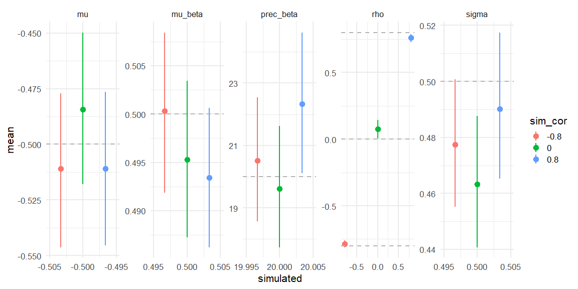
Here we see that all three models do recover the simulated parameters (inside the 90% HDI) (values depicted as the grey line).
Further exploration
One might give three objections or point of further investigation.
The Simulations above are not conditional on experimentally manipulated variables. Thus in order for this to be useful we need to show that we can recover parameters from the marginal distributions that are conditional on experimentally manipulated variables (X).
The Second objection is that for now this has only been done for continuous probability distributions. In order for this to be versatile we need to show that we can do the same for discrete probability distributions such as possion and binominal random variables.
The Third is that these these implementations are purely in a single subject framework and needs to be tested hierarchically, I.e. estimation subject level parameters nested within a group.
These steps are implemented in the next 3-markdowns!