
Discrete Confidence
Published:
- Multivariate Copula Modeling
This R markdown is for Showcasing the continous gaussian copula in non-gaussian marginals.
Table of content
Packages and setup
packages = c("brms","tidyverse","bayesplot",
             "pracma","here", "patchwork",
             "posterior","HDInterval","ordbetareg",
             "loo", "furrr","cmdstanr","mnormt","Rlab")


do.call(pacman::p_load, as.list(packages))

knitr::opts_chunk$set(echo = TRUE)

register_knitr_engine(override = FALSE)

set.seed(12345)
Overview.
Now that we have build multivariate models of three response types, i want to show and extend this to cases of discrete confidence ratings as many metacognitive experiments use these. To do this we need to make sure that both the binary responses and the confidence ratings are properly sampled. As for the binary responses we need to use the latent data-augmentation approach. Here I’ll go through how this can be done for confidence ratings that are discrete i.e. c ∈ {1, 2, 3, …K} but also ordered such that a confidence of 3 is higher than that of 2, and 2 higher than 1.
Ordered Logistic Regression and Latent Data Augmentation
The ordered logistic model is particularly suited for ordinal data like confidence ratings. The key insight is that we can think of the observed discrete confidence ratings as arising from an underlying continuous latent variable that is partitioned by cutpoints (also called thresholds).
The Ordered Logistic Model
For confidence ratings c ∈ {1, 2, 3, …K}, we use K − 1 cutpoints denoted as κ = (κ1, κ2, …, κK − 1) that divide the real line into K regions. These cutpoints must be ordered such that:
−∞ < κ1 < κ2 < … < κK − 1 < ∞
The probability that confidence equals category k is then defined as:
P(c = k) = P(κk − 1 < c* ≤ κk)
where c* is the underlying continuous latent variable, and we define κ0 = −∞ and κK = ∞ as boundary conditions.
For the ordered logistic specifically, this latent variable c* follows a logistic distribution (though one could use a normal distribution for ordered probit). The cumulative distribution function (CDF) of the logistic distribution is:
\[F(c^\*) = \frac{1}{1 + e^{-c^\*}}\]This means the probability of observing confidence category k is:
P(c = k) = F(κk) − F(κk − 1)
Latent Data Augmentation for Copulas
To use this in a copula framework, we need to extract uniform variables from our discrete confidence ratings. Similar to the binary case, we cannot simply apply the CDF because discrete distributions have stepwise CDFs that aren’t invertible. Instead, we use latent data augmentation.
The general idea is that the uniform variables that we extract from the discrete confidence ratings will have upper and lower bounds defined based on the ordered logistic CDF. For each observed confidence rating cn, we define bounds for the corresponding uniform variable Un such that:
Un ∼ Uniform(un−, un+)
where the bounds are:
\[u_n^- = F(\kappa_{c_n-1}) = \frac{1}{1 + e^{-\kappa_{c_n-1}}} \\ u_n^+ = F(\kappa_{c_n}) = \frac{1}{1 + e^{-\kappa_{c_n}}}\]4-Point Confidence Scale
Let’s make this concrete with a 3-point confidence scale where c ∈ {1, 2, 3}. We need K − 1 = 2 cutpoints: κ1, κ2.
If c = 1 (lowest confidence): \(u^- = F(\kappa_0) = F(-\infty) = 0 \\ u^+ = F(\kappa_1) = \frac{1}{1 + e^{-\kappa_1}}\)
If c = 2: \(u^- = F(\kappa_1) = \frac{1}{1 + e^{-\kappa_1}} \\ u^+ = F(\kappa_2) = \frac{1}{1 + e^{-\kappa_2}}\)
If c = 3: \(u^- = F(\kappa_2) = \frac{1}{1 + e^{-\kappa_2}} \\ u^+ = F(\kappa_K) = F(\infty) = 1\)
Notice how the intervals partition the [0, 1] interval completely, ensuring that Un remains uniformly distributed over [0, 1] marginally, while respecting the ordinal structure of the confidence ratings.
Extensions with Predictors
The ordered logistic model can also include predictors. If we have a linear predictor η = X**β, then the latent variable becomes c* = η + ϵ where ϵ follows a logistic distribution. The cutpoints remain fixed (though they can be made to vary with predictors in more complex models), and the probability becomes:
| P(c = k | X) = F(κk − η) − F(κk − 1 − η) |
This shifts the effective location of the cutpoints based on the predictor values, allowing different individuals or conditions to have different probabilities for each confidence category.
In the implementation below, we’ll show how to incorporate this latent data augmentation into a Stan model for jointly modeling binary decisions and discrete confidence ratings using a Gaussian copula.
simulate
qord_logit <- function(u, cutpoints) {
  cum_p <- plogis(cutpoints)

  y <- numeric(length(u))

  for (i in seq_along(u)) {
    # Find which category this u belongs to
    category <- 1
    for (k in seq_along(cum_p)) {
      if (u[i] >= cum_p[k]) {
        category <- k + 1
      } else {
        break
      }
    }
    y[i] <- category
  }

  return(y)
}


get_responses = function(rho){

  cutpoints = c(-0.5,0.5)


  df = data.frame(mnormt::rmnorm(n = 500, mean = c(0,0),
                       varcov = cbind(c(1,rho),c(rho,1)))) %>% rename(Bin = X1, RT = X2)

  uni_bin = pnorm(df$Bin)
  uni_RT = pnorm(df$RT)

  RT = qnorm(uni_RT,2,0.2)
  Bin = qord_logit(uni_bin,cutpoints = cutpoints)

  plot_pxy = data.frame(Bin = Bin, RT = RT) %>% ggplot() +
    geom_point(aes(x = Bin,y = RT), size = 0.5)+
    theme_minimal()+
    ggtitle(paste0("p(Bin,RT) at rho = ",rho))+
     theme(
      plot.title = element_text(size = 20),  # Increase title text size
      axis.title = element_text(size = 16), # Increase axis titles text size
      axis.text = element_text(size = 14)   # Increase axis tick text size
    )


plot_pxy

return(list(plot = plot_pxy, data = data.frame(Bin = Bin, RT = RT, cor = rho)))

}

functions {
  real gauss_copula_cholesky_lpdf(matrix u, matrix L) {
    array[rows(u)] row_vector[cols(u)] q;
    for (n in 1:rows(u)) {
      q[n] = inv_Phi(u[n]);
    }

    return multi_normal_cholesky_lpdf(q | rep_row_vector(0, cols(L)), L)
            - std_normal_lpdf(to_vector(to_matrix(q)));
  }

matrix uvar_bounds(array[] int binom_y, vector cutpoints, int is_upper) {
  int N = size(binom_y);
  int K = size(cutpoints) + 1;  // Number of categories
  matrix[N, 1] u_bounds;

  for (n in 1:N) {
    int y = binom_y[n];

    if (is_upper == 0) {  // Lower bound
      if (y == 1) {
        u_bounds[n, 1] = 0.0;
      } else {
        u_bounds[n, 1] = inv_logit(cutpoints[y - 1]);
      }
    } else {  // Upper bound
      if (y == K) {
        u_bounds[n, 1] = 1.0;
      } else {
        u_bounds[n, 1] = inv_logit(cutpoints[y]);
      }
    }
  }

  return u_bounds;
}

}

data {
  int<lower=0> N;
  vector[N] Y_con;
  array[N] int binom_y;
  int K;

}

parameters {
  ordered[K-1] cutpoints;
  real mu;
  real<lower=0> sigma;

  matrix<
    lower=uvar_bounds(binom_y, cutpoints, 0),
    upper=uvar_bounds(binom_y, cutpoints, 1)
    >[N, 1] u;

  cholesky_factor_corr[2] rho_chol;


}

model {
  matrix[N, 2] u_mix;

  for (n in 1:N) {
    u_mix[n, 1] = u[n,1];
    u_mix[n, 2] = normal_cdf(Y_con[n] | mu,sigma);
  }

  Y_con ~ normal(mu,sigma);

  u_mix ~ gauss_copula_cholesky(rho_chol);

  mu ~ normal(0,3);
  sigma ~ normal(0,3);
  cutpoints ~ normal(0,2);

  rho_chol ~ lkj_corr_cholesky(2);           // LKJ prior on correlation matrix


}

generated quantities {
  real rho = multiply_lower_tri_self_transpose(rho_chol)[1, 2];
}

corm08 = get_responses(-0.8)
cor0 = get_responses(0)
cor08 = get_responses(0.8)

datastan_corm08 = list(binom_y = corm08$data$Bin,
                       Y_con = corm08$data$RT,
                       K = 3,
                       N = nrow(corm08$data))


fit_corm08 = mixture_copula$sample(data = datastan_corm08,
                        refresh = 0,
                        iter_warmup = 500,
                        iter_sampling = 500,
                        parallel_chains = 4)
Displaying if we can recover!
parameters = c("cutpoints","mu","sigma","rho")

data = rbind(data.frame(fit_corm08$summary(parameters)) %>% mutate(simulated = c(-0.5,0.5,2,0.2,-0.8), sim_cor = -0.8),
             data.frame(fit_cor0$summary(parameters)) %>% mutate(simulated = c(-0.5,0.5,2,0.2,0), sim_cor = 0),
             data.frame(fit_cor08$summary(parameters)) %>% mutate(simulated = c(-0.5,0.5,2,0.2,0.8), sim_cor = 0.8))


data %>%
  mutate(sim_cor = as.factor(sim_cor)) %>%
  ggplot(aes(x = simulated, y = mean, ymin = q5, ymax = q95, col = sim_cor))+
  geom_pointrange(position=position_dodge(width=0.01))+
  facet_wrap(~variable,scales = "free", nrow = 1)+
  theme_minimal(base_size = 16)+
  geom_hline(aes(yintercept = simulated), data = data,
                color = "grey70", linetype = "dashed")+
  scale_x_continuous(breaks = scales::pretty_breaks(n = 3))
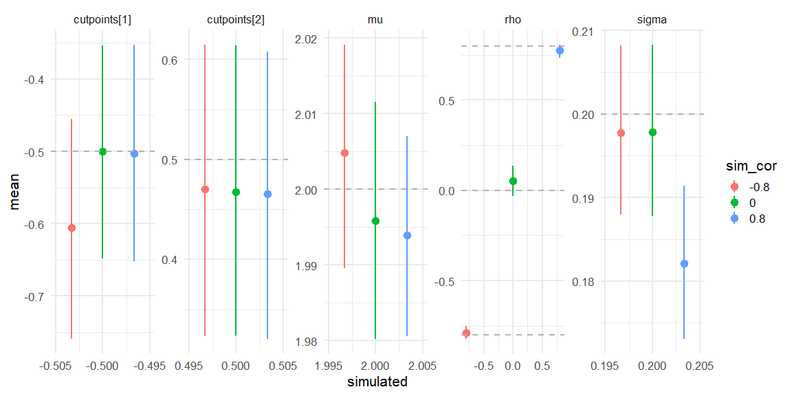
Here we see that all three models do recover the simulated parameters (inside the 90% HDI) (values depicted as the grey line).