
Discrete Copulas
Published:
- Multivariate Copula Modeling
This R markdown is for Showcasing of mixed marginals (continous and discrete) with a gaussian copula.
Table of content
- Overview
- Bernoulli and Gaussian marginals with a Gaussian copula.
- Simulation and fitting
- Further exploration
Packages and setup
packages = c("brms","tidyverse","bayesplot",
             "pracma","here", "patchwork",
             "posterior","HDInterval",
             "loo", "furrr","cmdstanr","mnormt","Rlab")


do.call(pacman::p_load, as.list(packages))

knitr::opts_chunk$set(echo = TRUE)

register_knitr_engine(override = FALSE)

set.seed(123)
Overview.
In this markdown the goal is to build on the previous markdowns, here i want to showcase how one can use the gaussian copula in the case of a binary and a continous maginal (say a bernoulli and gaussian).
Bernoulli and Gaussian marginals with a Gaussian copula.
Say we observe some binary responses (0,1) and some normally distributed response times (RT). We will in the following show how we can jointly model this combination.
First we want to simulate the situation and to do this we again start with a Gaussian copula with correlation coefficient ρ, then making these draws uniform with the guassian CDF and lastly using the inverse cumulative distributions of the distribution we want our binary responses and RT random variables to be drawn from (the “observed” responses).
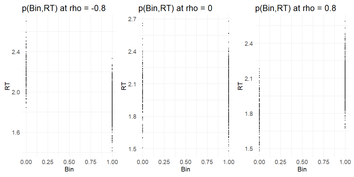
We are going to do this for 3 cases, highly positive dependency ρ = 0.8, no dependency ρ = 0 and , no highly negative dependency ρ = −0.8. For simplicity we will assume that there is a fixed probability of the binary response of being 1 i.e. θ = 0.7 while for the RT’s we assume a Normal distribution with μ = 2 σ = 0.2
Before showing the implementation we need to think carefully about how to implement this, because the Cummulative density functions of discrete variables are stepwise such that multiple values map unto the same cummulative probability. This makes the mapping not invertible and meaning there wont be a unique mapping from the uniform-variables to the discrete space. The implementation for overcoming this is that of data-augmentation, as highlighted here and in this paper.
The general idea is that the uniform variables that we have to extract from the discrete random variables will have upper and lower bounds that we define based on the CDF. Thus for the above case we will have some discrete random variable X = (X1, X2, Xn) for simplicity lets say that X ∈ (0, 1). What we now want to do is take the Cummulative density function of X to get the uniform variable U i.e.
Un = F(Xn) The clever way to do this is to set bounds for Un such that Un ∼ Uniform(un−, un+) where the bounds are defined from the marginal cummulative distribution function.
\[u_n^- = F(X_n-1) \\ u_n^+ = F(X_n)\]Thus for the Simplest case of the Bernoulli distribution we have a lower and upper bound for when Y = 0 and a lower and upper bound for when Y = 1, these are:
If Y = 0 \(u_n^- = F(0-1) = F(-1) = 0 \\ u_n^+ = F(0) = 1-\theta \\\) When Y = 1 we have: \(u_n^- = F(1-1) = F(0) = 1-\theta \\ u_n^+ = F(1) = 1 \\\) This will ensure that Un is uniform on each of the intervals which here one can see spans from 0 to 1 i.e. Un ∼ Uniform(0, 1).
# Making the function to do the above:

get_responses = function(rho){

  df = data.frame(mnormt::rmnorm(n = 500, mean = c(0,0),
                       varcov = cbind(c(1,rho),c(rho,1)))) %>% rename(VAS = X1, RT = X2)

  uni_bin = pnorm(df$VAS)
  uni_RT = pnorm(df$RT)


  Bin = qbern(uni_bin,p = 0.7)
  RT = qnorm(uni_RT,2,0.2)

  plot_pxy = data.frame(Bin = Bin, RT = RT) %>% ggplot() +
    geom_point(aes(x = Bin,y = RT), size = 0.5)+
    theme_minimal()+
    ggtitle(paste0("p(Bin,RT) at rho = ",rho))+
     theme(
      plot.title = element_text(size = 20),  # Increase title text size
      axis.title = element_text(size = 16), # Increase axis titles text size
      axis.text = element_text(size = 14)   # Increase axis tick text size
    )


plot_pxy

return(list(plot = plot_pxy, data = data.frame(Bin = Bin, RT = RT, cor = rho)))

}
Plotting the results of using the function at the level of the response variables (i.e. Ratings and response times)
get_responses(-0.8)[[1]]+get_responses(0)[[1]]+get_responses(0.8)[[1]]
Now we have data that kind of looks like something from an experiment the question is can we recover the parameters we put in? In order to do this we write the stan model:
functions {
  real gauss_copula_cholesky_lpdf(matrix u, matrix L) {
    array[rows(u)] row_vector[cols(u)] q;
    for (n in 1:rows(u)) {
      q[n] = inv_Phi(u[n]);
    }

    return multi_normal_cholesky_lpdf(q | rep_row_vector(0, cols(L)), L)
            - std_normal_lpdf(to_vector(to_matrix(q)));
  }


  matrix uvar_bounds(array[] int binom_y, real theta, int is_upper) {

    int N = size(binom_y);
    matrix[N, 1] u_bounds;

    //go through all the trials
    for (n in 1:N) {
      //is the lower bound returned?
      if (is_upper == 0) {
        // if the bernoulli random variable is 0 return 0,
        // if its not 0 (i.e. 1), then return binomial_cdf(0 | 1, theta) (equvilent to bernoulli_CDF(0 |theta)) which is (1-theta)

        u_bounds[n, 1] = binom_y[n] == 0.0 ? 0.0 : binomial_cdf(binom_y[n] - 1 | 1, theta);

      //if we want the upper bound
      } else {
        // If random variable is 0 we again return (1-theta) as the above,
        // If its 1 however then we get binomial_cdf(1|1,theta) or (bernoulli_CDF(1 |theta)) which is just 1.
        u_bounds[n, 1] = binomial_cdf(binom_y[n] | 1, theta);
      }
    }

    return u_bounds;
  }


}

data {
  int<lower=0> N;
  vector[N] Y_con;
  array[N] int binom_y;
}

parameters {
  real<lower=0, upper = 1> theta;
  real mu;
  real<lower=0> sigma;

  matrix<
    lower=uvar_bounds(binom_y, theta, 0),
    upper=uvar_bounds(binom_y, theta, 1)
    >[N, 1] u;

  cholesky_factor_corr[2] rho_chol;


}

model {
  matrix[N, 2] u_mix;

  for (n in 1:N) {
    u_mix[n, 1] = u[n,1];
    u_mix[n, 2] = normal_cdf(Y_con[n] | mu,sigma);
  }

  Y_con ~ normal(mu,sigma);

  u_mix ~ gauss_copula_cholesky(rho_chol);

  mu ~ normal(0,3);
  sigma ~ normal(0,3);
  theta ~ normal(0,1);

  rho_chol ~ lkj_corr_cholesky(2);           // LKJ prior on correlation matrix


}

generated quantities {
  real rho = multiply_lower_tri_self_transpose(rho_chol)[1, 2];
}
Displaying if we can recover!
parameters = c("theta","mu","sigma","rho")

data = rbind(data.frame(fit_corm08$summary(parameters)) %>% mutate(simulated = c(0.7,2,0.2,-0.8), sim_cor = -0.8),
             data.frame(fit_cor0$summary(parameters)) %>% mutate(simulated = c(0.7,2,0.2,0), sim_cor = 0),
             data.frame(fit_cor08$summary(parameters)) %>% mutate(simulated = c(0.7,2,0.2,0.8), sim_cor = 0.8))


data %>%
  mutate(sim_cor = as.factor(sim_cor)) %>%
  ggplot(aes(x = simulated, y = mean, ymin = q5, ymax = q95, col = sim_cor))+
  geom_pointrange(position=position_dodge(width=0.01))+
  facet_wrap(~variable,scales = "free", nrow = 1)+
  theme_minimal(base_size = 16)+
  geom_hline(aes(yintercept = simulated), data = data,
                color = "grey70", linetype = "dashed")+
  scale_x_continuous(breaks = scales::pretty_breaks(n = 3))
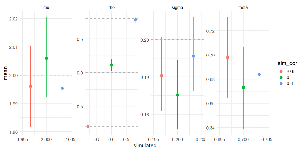
Here we see that all three models do recover the simulated parameters (inside the 90% HDI) (values depicted as the grey line).