Multivariate Normals

8 minute read

Published: February 01, 2025

Multivariate Copula Modeling

This R markdown is for explaining simple copula modeling in stan.

Table of content

Overview
Forward simulations
Stan Implementations
Fitting and Mutual Information
Conclusion

Packages and setup

packages = c("brms","tidyverse","bayesplot",
             "pracma","here", "patchwork",
             "posterior","HDInterval",
             "loo", "furrr","cmdstanr","mnormt")


do.call(pacman::p_load, as.list(packages))

knitr::opts_chunk$set(echo = TRUE)

register_knitr_engine(override = FALSE)

set.seed(123)

Overview.

In this markdown the goals is to build up an understanding of multivariate distributions. I will introduce this with Gaussian random variables. In this markdown I will show that there are 3 different ways of simulating such that two of which are practically equvient whereas the last is just a special case of the two. The three types of models are:

Two marginal Gaussian (no off diagonal in the variance covariance matrix)
A multivariate Gaussian with a mean vector and a variance covariance matrix
Two marginal Gaussian with a gaussian copula linking the two marginals

Forward simulations

Two Marginal Gaussian Distributions without a variance covariance matrix

Two independent univariate Gaussian random variables can be written as:

That is,

\[\mathbf{Y} = \begin{bmatrix} Y_1 \\ Y_2 \end{bmatrix} \sim \mathcal{N} \left( \begin{bmatrix} \mu_1 \\ \mu_2 \end{bmatrix}, \begin{pmatrix} \sigma_1^2 & 0 \\ 0 & \sigma_2^2 \end{pmatrix} \right)\]

A multivariate Gaussian

\[\mathbf{Y} = \begin{bmatrix} Y_1 \\ Y_2 \end{bmatrix} \sim \mathcal{N} \left( \begin{bmatrix} \mu_1 \\ \mu_2 \end{bmatrix}, \begin{pmatrix} \sigma_1^2 & \sigma_1\sigma_2\rho \\ \sigma_1\sigma_2\rho & \sigma_2^2 \end{pmatrix} \right)\]

When ρ = 0, this reduces to the independent case above.

Two marginal Gaussian with a Gaussian copula

Starting from random variables with arbitrary marginals f₁ and f₂ (these are in this case two marginal normals) f₁ ∼ 𝒩(μ₁, σ₁) & f₁ ∼ 𝒩(μ₂, σ₂)

Mathematically this can be written as the two marginals

Y₁ ∼ f₁(θ₁)

Y₂ ∼ f₂(θ₂) To model the dependence we transform (Y₁, Y₂) into two uniforms through the probability integral transform. These are then back transformed into standard multivariate normal variables with correlation ρ this can be written in a single equation:

\[(z_1, z_2) = \begin{bmatrix} \Phi^{-1}\big(F_1(Y_1)\big) \\ \Phi^{-1}\big(F_2(Y_2)\big) \end{bmatrix} \sim \mathcal{N}\Bigg( \mathbf{0}, \begin{bmatrix} 1 & \rho \\ \rho & 1 \end{bmatrix} \Bigg), \quad F_i(\cdot) \text{ are the marginal CDFs}\]

This chain of transformations shows how arbitrary marginal distributions can be linked through a Gaussian copula, with ρ controlling the dependence between the marginals.

Using LOO we show that the multivariate and copula Gaussian for all ρ are no different, but both being being better for all ρ != 0 than the two marginal Gaussians

Stan Implementations

We thus start with the stancode for the 3 models:

2 Marginal Gaussians:

data {
  int<lower=1> N;             // Number of observations
  vector[N] y1;               // Outcome variable 1
  vector[N] y2;               // Outcome variable 2
}

parameters {
  vector[2] beta;         // Coefficients for y2
  vector<lower=0>[2] sigma;      // Standard deviations for y1 and y2

}

model {
  // Priors
  beta ~ normal(0, 10);
  sigma ~ normal(0, 5);

  for(i in 1:N){
    y1[i] ~ normal(beta[1], sigma[1]);
    y2[i] ~ normal(beta[2], sigma[2]);
  }
}
generated quantities{
  vector[N] log_lik = rep_vector(0,N);
  
    // Likelihood
  for (n in 1:N) {
    log_lik[n] += normal_lpdf(y1[n] | beta[1], sigma[1]);
    log_lik[n] += normal_lpdf(y2[n] | beta[2], sigma[2]);
  }
}

Multivariate Gaussian

data {
  int<lower=1> N;                // Number of observations
  matrix[N, 2] y;                // Observed outcomes [y1, y2]
}

parameters {
  vector[2] beta;         // Coefficients for y2
  vector<lower=0>[2] sigma;      // Standard deviations for y1 and y2
  corr_matrix[2] Omega;          // Correlation matrix
}

transformed parameters {
  cov_matrix[2] Sigma;           // Covariance matrix
  Sigma = quad_form_diag(Omega, sigma);
}

model {
  beta ~ normal(0, 10);
  sigma ~ normal(0, 5);
  Omega ~ lkj_corr(2);           // LKJ prior on correlation matrix
  // Likelihood
  for (n in 1:N) {
    y[n] ~ multi_normal(beta, Sigma);
  }
}

generated quantities{
  vector[N] log_lik;
  
    // Likelihood
  for (n in 1:N) {
    log_lik[n] = multi_normal_lpdf(y[n] | beta, Sigma);
  }
  
}

2 Marginal Gaussians and guassian copula:

functions {
  
  real gauss_copula_cholesky_lpdf(matrix u, matrix L) {
    array[rows(u)] row_vector[cols(u)] q;
    for (n in 1:rows(u)) {
      q[n] = inv_Phi(u[n]);
    }

    return multi_normal_cholesky_lpdf(q | rep_row_vector(0, cols(L)), L)
            - std_normal_lpdf(to_vector(to_matrix(q)));
  }
  
  vector gauss_copula_cholesky_per_row(matrix u, matrix L) {
    int N = rows(u);
    int D = cols(u);
    array[N] row_vector[D] q;
    vector[N] loglik;

    for (n in 1:N) {
        q[n,] = inv_Phi(u[n,]);
        loglik[n] = multi_normal_cholesky_lpdf(to_row_vector(q[n,]) | 
                                                 rep_row_vector(0, D), L) - std_normal_lpdf(to_vector(to_matrix(q[n,])));
    }

    return loglik;
  }
  
}

data {
  int<lower=0> N;
  matrix[N, 2] y;
}

parameters {
  real<lower=0> sigma1;
  real<lower=0> sigma2;
  real<lower=0> mu1;
  real<lower=0> mu2;
  
  cholesky_factor_corr[2] rho_chol;
}

transformed parameters{
  
  matrix[N, 2] u;
  
  for (n in 1:N) {
    u[n, 1] = normal_cdf(y[n, 1] | mu1,sigma1);
    u[n, 2] = normal_cdf(y[n, 2] | mu2,sigma2);
  }

}

model {
  
  mu1 ~ normal(0, 10);
  mu2 ~ normal(0, 10);
  
  sigma1 ~ normal(0, 5);
  sigma2 ~ normal(0, 5);
  
  rho_chol ~ lkj_corr_cholesky(2);

  y[, 1] ~ normal(mu1,sigma1);
  y[, 2] ~ normal(mu2,sigma2);

  u ~ gauss_copula_cholesky(rho_chol);
}

generated quantities {
  real rho = multiply_lower_tri_self_transpose(rho_chol)[1, 2];
  vector[N] log_lik;  // per-trial log-likelihood

  matrix[2,2] Sigma = multiply_lower_tri_self_transpose(rho_chol);


  vector[N] ll_copula = gauss_copula_cholesky_per_row(u, rho_chol);
  
  
  for (n in 1:N) {
    // Marginal contributions
    real ll_marg = normal_lpdf(y[n,1] | mu1, sigma1) + normal_lpdf(y[n,2] | mu2, sigma2);

    
    // Total per-trial log-likelihood
    log_lik[n] = ll_marg + ll_copula[n];
  }
}

Fitting and Mutual Information

Now we simulate some multivariate data with correlation coefficient r, and then fit each of the stan models. Furthermore we can compare how well the stanmodels fit the data, but computing approximate leave one out crossvalidation (LOO-CV).

# Set up parallel plan
plan(multisession, workers = 10)  # Adjust to your number of cores

# Correlations to simulate
r = seq(-0.6, 0.6, by = 0.05)

# Function to simulate and fit models for one correlation
simulate_and_fit <- function(cor) {
  
  # Simulate data
  n_out <- mnormt::rmnorm(n = 500, mean = c(1, 2),
                          varcov = cbind(c(1, cor), c(cor, 1)))
  
  bdata <- data.frame(
    y1 = n_out[,1],
    y2 = n_out[,2]
  )
  
  # Marginal model
  datastan_margin <- list(
    y1 = bdata$y1,
    y2 = bdata$y2,
    N = nrow(bdata)
  )
  
  fit_margin <- marginal$sample(
    data = datastan_margin,
    refresh = 0,
    adapt_delta = 0.99,
    parallel_chains = 4
  )
  
  # Multivariate & copula models
  datastan_multi <- list(
    y = cbind(bdata$y1, bdata$y2),
    N = nrow(bdata)
  )
  
  fit_multi <- multivariate$sample(
    data = datastan_multi,
    refresh = 0,
    adapt_delta = 0.99,
    parallel_chains = 4
  )
  
  fit_cor <- copula$sample(
    data = datastan_multi,
    refresh = 0,
    adapt_delta = 0.99,
    parallel_chains = 4
  )
  
  # Compute LOO comparison
  loo_df <- data.frame(
    loo::loo_compare(
      list(
        margin = fit_margin$loo(),
        corpula = fit_cor$loo(),
        multi = fit_multi$loo()
      )
    )
  ) %>% rownames_to_column()
  
  loo_df$sim_correlation <- cor
  
  return(list(loo_df,fit_margin,fit_cor,fit_multi))
}

# Run in parallel and combine results directly
loos <- future_map(r, simulate_and_fit, .progress = T)

Now we can plot the results of these model comparisons:

Plottiing the results of this

plot = map_dfr(loos,1) %>% filter(elpd_diff != 0) %>% mutate(models = rowname) %>% 
  ggplot()+
  geom_pointrange(aes(x = sim_correlation, y = elpd_diff, ymin = elpd_diff-2*se_diff, ymax = elpd_diff+2*se_diff, col = models))+
  theme_minimal()+
  theme(legend.position = "top")+
  theme(text = element_text(size = 24))+
  scale_x_continuous(breaks = seq(-0.8,0.8,by = 0.1), labels = seq(-0.8,0.8,by = 0.1))

plot

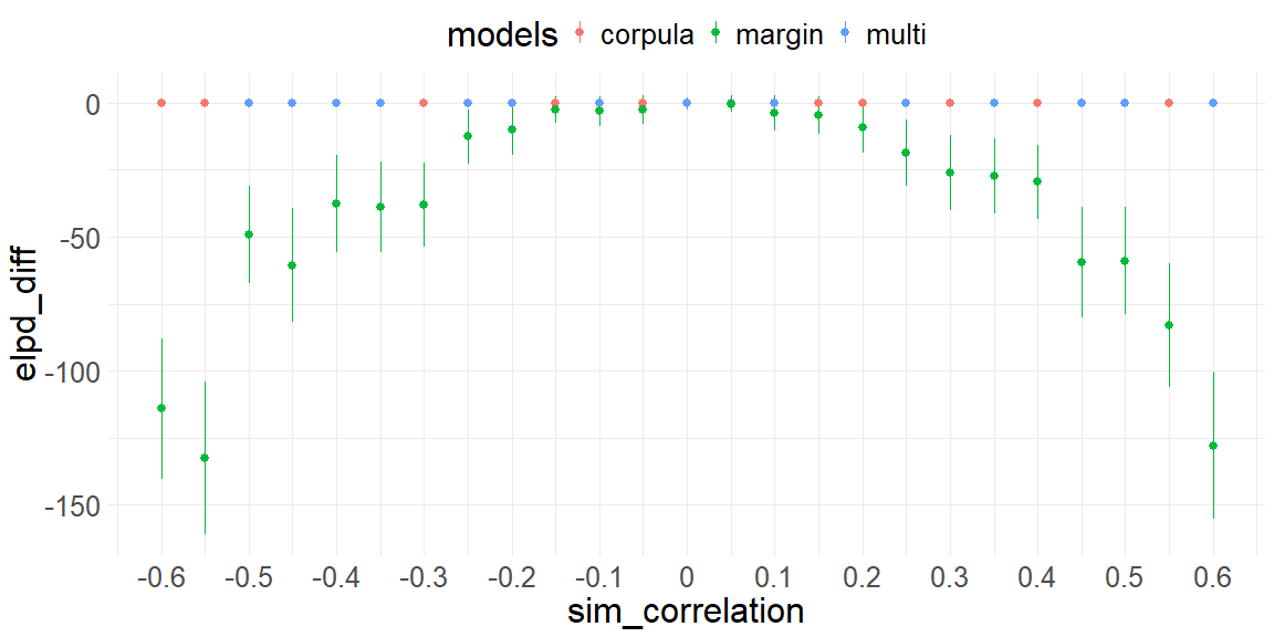
Simulation results showing LOO-CV performance

This figure shows the simulation results of 500 trials per simulation of correlation coefficients ((-0.6 ; 0.6 , by = 0.06) x-axis) of three models (colors) on their performance of LOO-CV. The plot shows how the marginal implementation explains the data worse in a quadratic way with respect to the simulated correlation coefficient. Furthermore, the copula and multivariate implementation share to explain the data the best (randomly alternating blue and red colors at elpd_diff = 0).

This shows that our implementation of the Gaussian copula is at least sensible because it behaves in exactly the same way as the multivariate normal. Further this simulation shows that the degree to which we explain the data worse with the marginal implementation is quadratic on the correlation coefficient. This is of course not a coincidence and is evident if we write the mutual information of our two random variables:

\[MI(x, y) \leq \frac{1}{2} \log \left( \frac{1}{1 - r^2} \right)\]

this quantity is measured in bits. The interesting part is that it depends on the square of the correlation coefficient. Which aligns with the plot above, when plotted ontop with a scaling factor of the sample size we see:

plot+geom_line(data = data.frame(),aes(x = r, y = (-1/2*log(1/(1-r^2)) * 500)))

Mutual information comparison

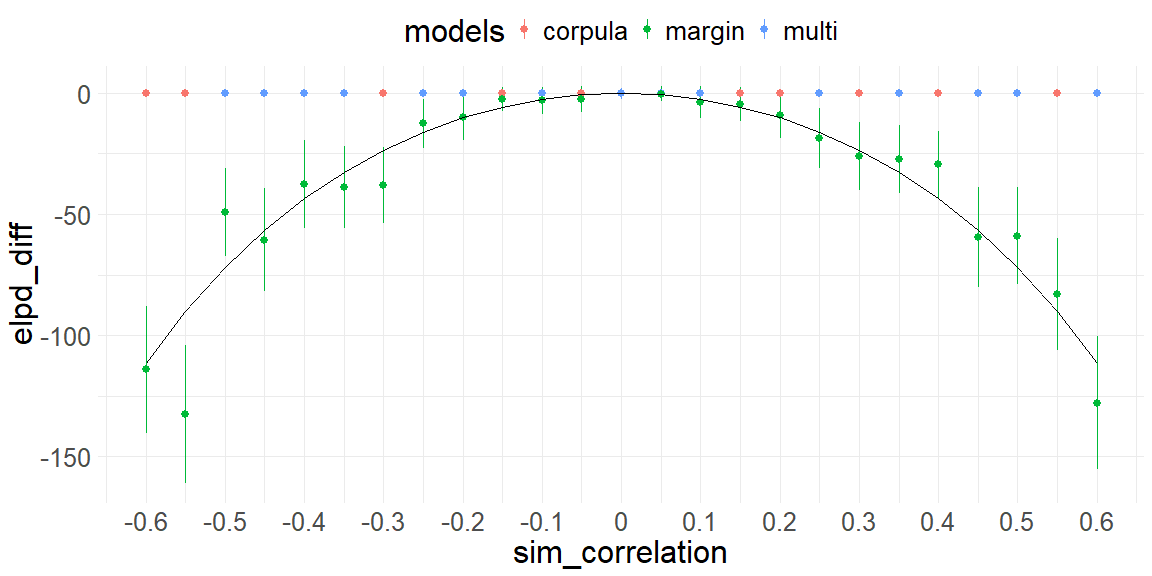
In short, we can implement and showcase that the copula implementation works when comparing guassian distributions and correlation coefficients and guassian copulas and that the LOO-CV captures the underlying relationship. Next, the strength of the copula implementations will be showcased, that is when the two marginals aren’t Gaussian.

Conclusion

Share on

X (formerly Twitter) Facebook LinkedIn

Jesper Fischer Ehmsen