2 Part 2: Current Model
In this section, we first describe the general structure of ideas of static models of perceptual decision making and confidence ratings. We then describe, derive and simulate from our proposed model, demonstrating that it can produce key patterns of perceptual decision making with confidence judgements.
2.1 Static models of metacognition
In SDT, an actor makes a binary choice on each trial \(i\), \(a_i \in \{-1,+1\}\) based on some internal evidence \(e_i\). The action reflects the actor’s inference about the true state of the stimulus \(D_i \in \{-1,+1\}\).
Evidence is drawn from a normal distribution, reflecting the noisy nature of perception. The mean of this distribution reflects the true state and scales with stimulus intensity \(X_i\). \[ e_i \sim \mathcal{N}(X_iD_i,\sigma_e) \]
The actor then produces an action by comparing the internal evidence to a criterion \(c\):
\[ a_i = \begin{cases}+1 & \text{if } e_i > c \\ -1 & \text{if } e_i \le c\end{cases} \]
Within most frameworks, this criterion is thought to be static within an experimental setting for each agent.
2.1.1 Confidence Ratings
Having made a binary choice, the agent is asked to give a confidence judgement in that choice. A prominent approach is to assume that the agent computes the probability that the action was correct. Fleming and Daw (2017) extended this framework to also account for error monitoring.
In their formulation, the confidence judgement is based on a set of variables drawn from a multivariate normal: the evidence used for the action \(e_i\) and a pseudo-independent information accessible only to the rater \(r_i\). These two quantities are correlated, with \(\rho\) governing information sharing. If \(\rho\) = 1, the confidence judgement is based on the same information as the action; if \(\rho\) = 0, it is based on completely independent information.
\[ \begin{bmatrix}e_i \\ r_i\end{bmatrix}\sim \mathcal{N}\left(\begin{bmatrix}X_iD_i \\ X_iD_i\end{bmatrix},\begin{bmatrix}\sigma_e^2 & \rho \cdot \sigma_e \cdot \sigma_m \\ \rho \cdot \sigma_e \cdot \sigma_m & \sigma_m^2\end{bmatrix}\right) \]
The rater then uses this information to compute the subjective probability of being correct, which generates a confidence rating. A central argument for models with independent information is their ability to explain error monitoring: agents sometimes recognize that they have made an error and give low (even below-chance) confidence ratings. The need for independent information follows from the fact that a rational agent who bases both choice and confidence on the same information (i.e., \(\rho = 1\) in the above model), and whose choices are deterministic, cannot make an error while being aware of it. Any information indicating that the choice is incorrect would also determine the choice itself, thereby preventing the error.
2.2 Efference copy (Choice Variability) model of metacognition (EA/CV - Meta)
2.2.1 Choices
Below we argue that independent information is not required to explain error monitoring if we instead assume that agents show variability in their choices given the evidence. Unlike the deterministic decision policy usually assumed in SDT, we propose that agents have a noisy decision process that can produce errors even when the evidence favors the correct choice. Such errors could arise under speed stress or, more generally, from motor noise. By introducing a stochastic choice policy into the standard SDT framework, agents can display error monitoring without independent information. One way to implement this is to assume that the criterion varies from trial to trial: \(c_i \sim \mathcal{N}(0,\sigma_c)\). This gives us:
\[ a_i = \begin{cases}+1 & \text{if } e_i > c_i \\ -1 & \text{if } e_i \le c_i\end{cases} \]
Because both \(e_i\) and \(c_i\) are normally distributed, their difference is also normally distributed and can be marginalized to obtain the probability of the action:
\[ P(a = 1 \mid D_i, X_i) = \Phi\left(\frac{D_i \cdot X_i}{\sqrt{\sigma_e^2 + \sigma_c^2}}\right) \]
Before moving on to confidence ratings, we will also assume that the evidence distribution may be biased for each participant. This assumption helps explain the observation that shifts in the psychometric function of choices are accompanied by corresponding shifts in other behavioral variables such as confidence ratings (Caziot and Mamassian 2021; Sánchez-Fuenzalida et al. 2025; Mihali et al. 2023; Navajas et al. 2017).
This leads to:
\[ e_i \sim \mathcal{N}(X_iD_i- \beta,\sigma_e) \] And when marginalized:
\[ P(a = 1 \mid D_i, X_i) = \Phi\left(\frac{D_i \cdot X_i - \beta}{\sqrt{\sigma_e^2 + \sigma_c^2}}\right) \tag{1} \]
From choices alone, only the sum \(\sigma_e^2 + \sigma_c^2\) can be identified, as both noise sources equivalently flatten the psychometric function. However, including confidence ratings allows the two to be disentangled.
2.2.2 Confidence ratings
To compute confidence ratings, we assume that the agent internally computes the subjective probability that the choice was correct.
\[ \text{confidence} = P(\text{correct} \mid r, a) = P(D = a \mid r) \]
Here we assume that the rater has access to a noisy readout of the evidence: \(r_i \sim \mathcal{N}(e_i, \sigma_m)\), where \(\sigma_m\) is metacognitive noise.
This can be shown to yield: (see the full derivation see below):
Click to expand: Derivation of the probability of correctness given noisy evidence.
If we assume, as Signal detection theory, that the evidence is Gaussian, we can write:
\[ e \sim \mathcal{N}(D \cdot X_i, \sigma_e) \]
We now assume that the agent computes the posterior probability of D given the evidence he collected. This means that for the case where D = 1 we have from bayes theorm that:
\[ P(D=1 \mid e) = \frac{P(e \mid D=1) \cdot P(D=1)}{P(e \mid D=1) \cdot P(D=1) + P(e \mid D=-1) \cdot P(D=-1)} \]
where the prior probability of e is written as; \(p(e) = P(e \mid D=1) \cdot P(D=1) + P(e \mid D=-1) \cdot P(D=-1)\) due to the law of total probability.
This means that the posterior probability that the state of the world is 1 (dots moving right) given the evidence is just the likelihood of the evidence given that the state was 1 weighted by the prior of the stimulus, divided by the total probability.
If we now assume that the prior of the true state of the world is flat (i.e. P(D = 1) = P(D = -1) = 0.5). we have:
\[ P(D=1 \mid e) = \frac{P(e \mid D=1)}{P(e \mid D=1) + P(e \mid D=-1)} \]
Plugging in the Gaussian distributions from the assumption of the evidence:
\[ e \mid D=1 \sim \mathcal{N}(X_i, \sigma_e^2), \quad e \mid D=-1 \sim \mathcal{N}(-X_i, \sigma_e^2) \]
Then the likelihoods are:
\[ P(e \mid D=1) = \frac{1}{\sqrt{2\pi\sigma_e^2}} \exp\Big(-\frac{(e - X_i)^2}{2\sigma_e^2}\Big), \quad P(e \mid D=-1) = \frac{1}{\sqrt{2\pi\sigma_e^2}} \exp\Big(-\frac{(e + X_i)^2}{2\sigma_e^2}\Big) \]
Plugging these into the posterior formula:
\[ \begin{aligned} P(D=1 \mid e) &= \frac{\exp\Big(-\frac{(e - X_i)^2}{2\sigma_e^2}\Big)}{\exp\Big(-\frac{(e - X_i)^2}{2\sigma_e^2}\Big) + \exp\Big(-\frac{(e + X_i)^2}{2\sigma_e^2}\Big)} \end{aligned} \]
Now if one factors out the \(\exp\Big(-\frac{(e - X_i)^2}{2\sigma_e^2}\Big)\) term from the numerator we get:
\[ P(D=1 \mid e) = \frac{1}{1 + \exp\Big(\frac{(e + X_i)^2 - (e - X_i)^2}{2\sigma_e^2}\Big)} \] writing out the sqaures \((e + X_i)^2 = e^2 + X_i^2 + 2\cdot e \cdot X_i\) & \((e - X_i)^2 = e^2 + X_i^2 - 2\cdot e \cdot X_i\), we end up with:
\[ P(D=1 \mid e) = \frac{1}{1 + \exp\Big(-\frac{2 \cdot e \cdot X_i}{\sigma_e^2}\Big)} \] This type of fraction is exactly the inverse logit transformation \(g(.) = \frac{1}{1+exp(-x)}\), which means: \[ P(D=1 \mid e) = g\Big(\frac{2 \cdot e \cdot X_i}{\sigma_e^2}\Big) \]
\[ P(\text{correct} \mid r_i, a, X_i) = \begin{cases}g\left(\frac{2 \cdot r_i \cdot X_i}{\sigma_e^2 + \sigma_m^2}\right) & \text{if } a = 1 \\ 1 - g\left(\frac{2 \cdot r_i \cdot X_i}{\sigma_e^2 + \sigma_m^2}\right) & \text{if } a = -1\end{cases} \tag{2} \]
Here we assume a uniform prior on \(D\), i.e., \(P(D_i = 1) = P(D_i = -1) = 0.5\), representing the true state of the world (i.e. in the Random Dot Motion task, whether the dots are moving up or down).
Here \(g(\cdot)\) is the inverse logit transformation, i.e., \(g(x)= \frac{1}{1+exp(-x)}\).
From confidence alone, only the sum \(\sigma_e^2 + \sigma_m^2\) can be identified. However, combining choices and confidence allows estimation of all three parameters: \(\sigma_e\), \(\sigma_c\), and \(\sigma_m\).
As can be seen from equation (2), computing the probability of being correct requires access to the stimulus intensity \(X_i\). Although this is assumed in some models (Fleming et al. 2018), we believe the rater does not have access to the objective stimulus intensity. We return to this issue later, where note that we fix this quantity to one for the current registration. Interested readers are referred to Rausch and Zehetleitner (2019), where simulations are conducted with different generative processes for the stimulus intensity.
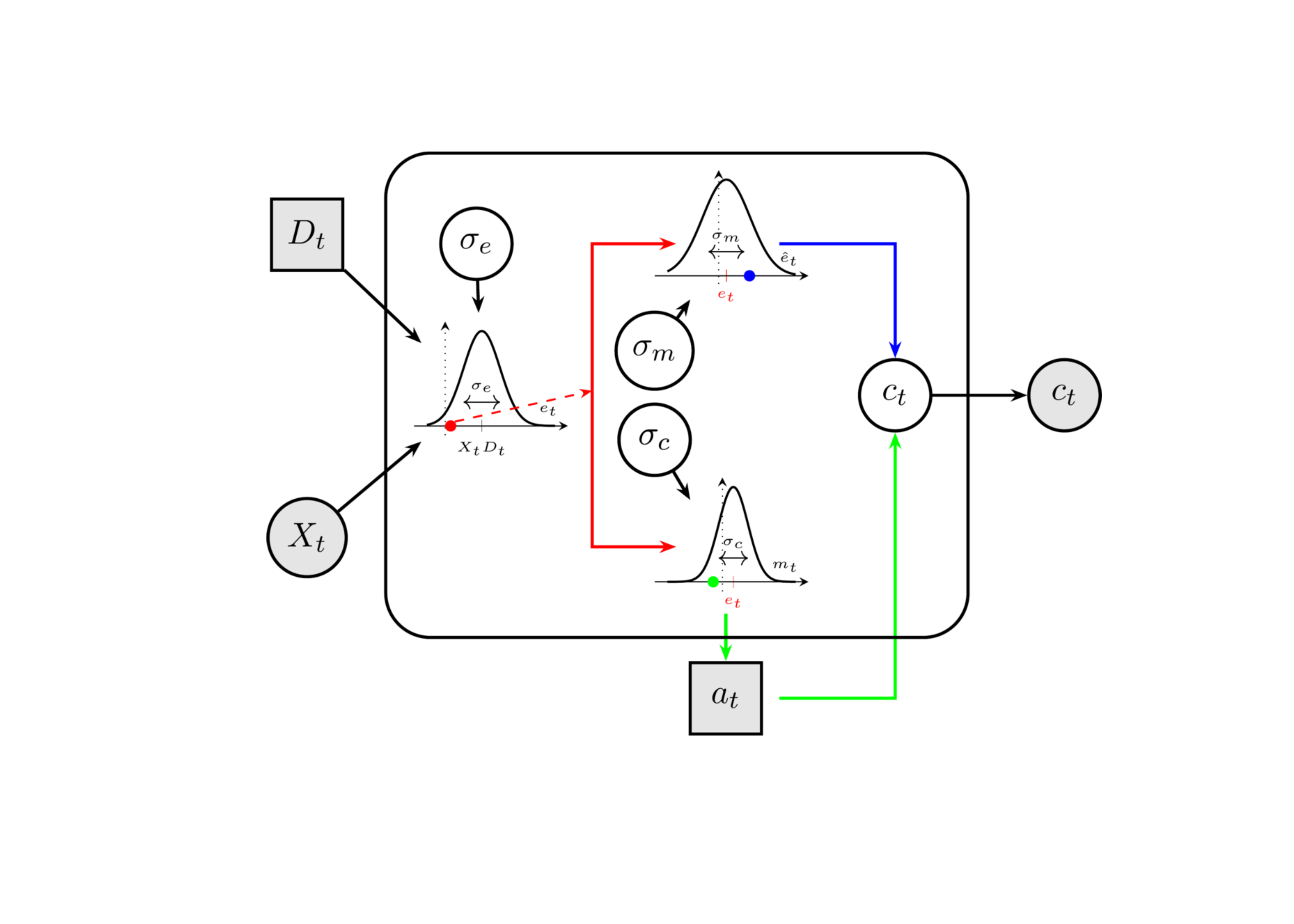
Below we present a plate notation schematic of the proposed model, illustrating the role of each noise parameter.
The model assumes that an agent is presented with a stimulus that has a direction \(D_i\) (the true state of the world) and a strength \(X_i\). An internal representation of the physical stimulus (evidence), \(e_i\) (red point), is a noisy readout of the physical stimulus. This internal evidence is then sent to the pre-motor and motor cortex, where an efferent signal and an efference copy are produced (red split path). Due to additional noise (\(\sigma_c\)) in the processing and transmission of the signal to the limb, the action generated may be opposite to what the evidence indicated (green point). Simultaneously, the efference copy may also be subject to additional noise (\(\sigma_m\)). It is then used together with the action to produce a prediction error in the comparator \(C_t\), which in turn generates the confidence rating.
Next, we present simulations from the model to build intuition about the parameters and their interact.
2.2.3 Simulations
Below we demonstrate that the model reproduces key behavioral patterns of choice and confidence ratings under different parameter combinations. In brief, our simulations show that the ratio \(\frac{\sigma_e}{\sigma_c}\) determines the degree of error monitoring and whether the confidence patterns is a folded-X or double-increase.
A low ratio (high \(\sigma_c\), low \(\sigma_e\)) produces folded-X (strong error monitoring), while a high ratio (low \(\sigma_c\), high \(\sigma_e\)) produces double-increase (no error monitoring).
The metacognitive noise \(\sigma_m\) flattens the confidence curves regardless of accuracy.
Note: For all simulations below, we assume that the bias in evidence encoding \(\beta\) is 0. We return to this issue later, in connection with the assumption about whether participants have access to the objective stimulus intensity.
First, we examine the distribution of internal evidence over the objective signed stimulus (i.e., the product of stimulus intensity and the true state) across the two parameters governing the choices; \(\sigma_e\) (evidence encoding ) and \(\sigma_c\) (choice variability).
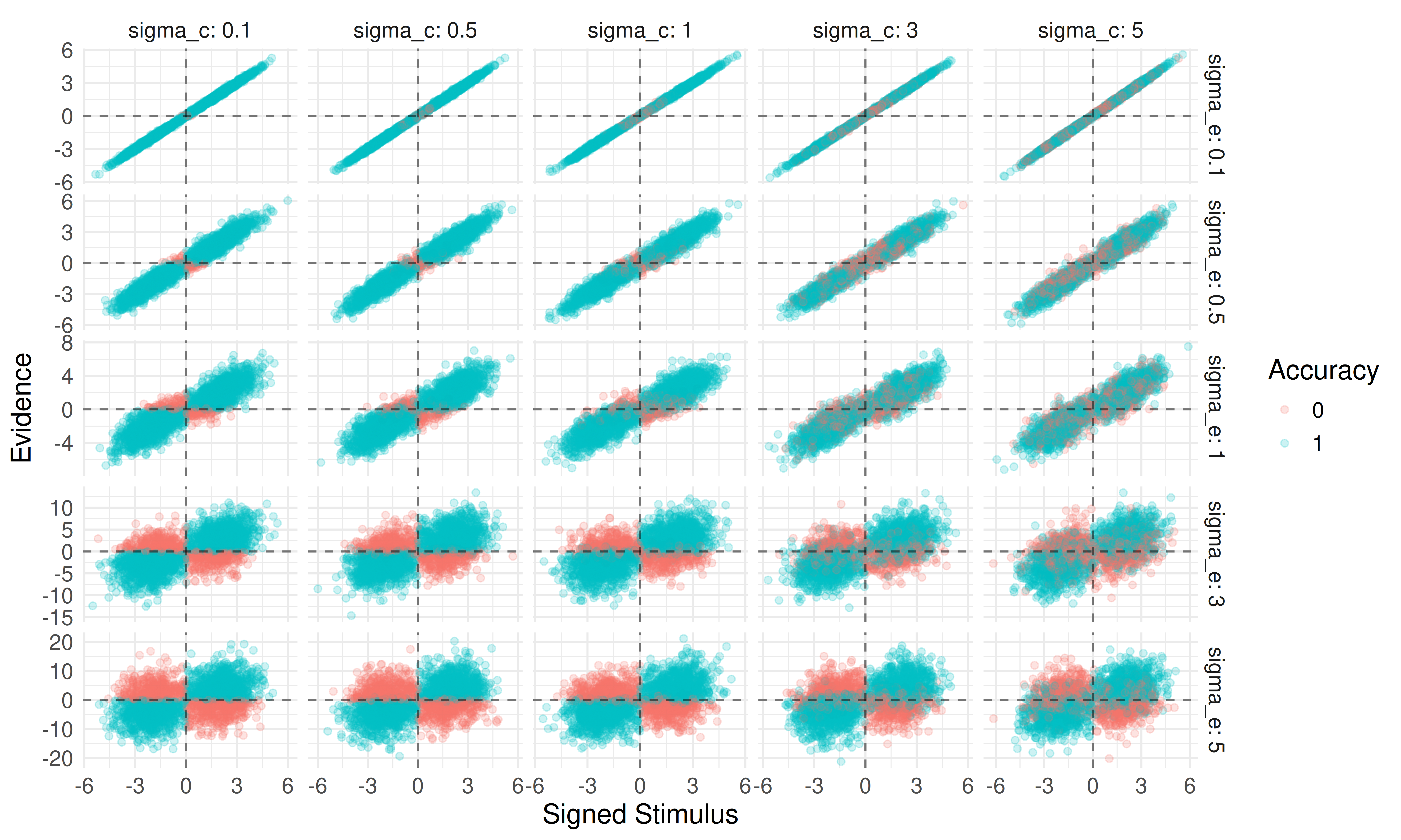
From the above plot we see that \(\sigma_e\) broadens the range of observed evidence (making it noisier for the same external stimulus); moving down the rows, the y-axis range greatly increases. When \(\sigma_c\) is low (left column), choices are consistent, positive evidence is paired with positive signed stimulus (i.e. D = 1), yielding a correct response. As \(\sigma_c\) increases this relationship becomes noisier, and correct and incorrect choices become less distinguishable across the zero-evidence line and zero-signed-stimulus lines.
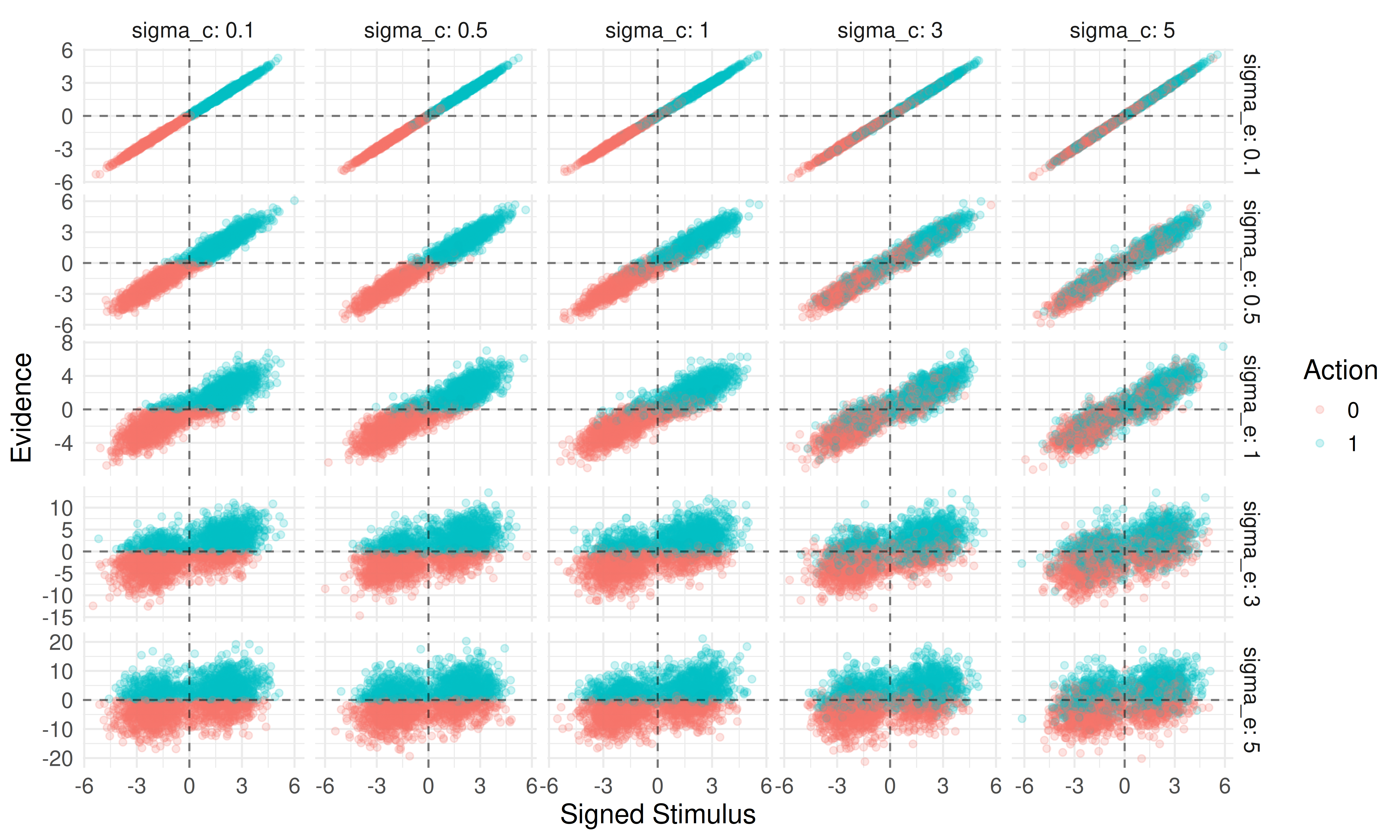
Another way to display this is by plotting actions instead of accuracy:
Next, we examine confidence ratings as a function of the three noise parameters.
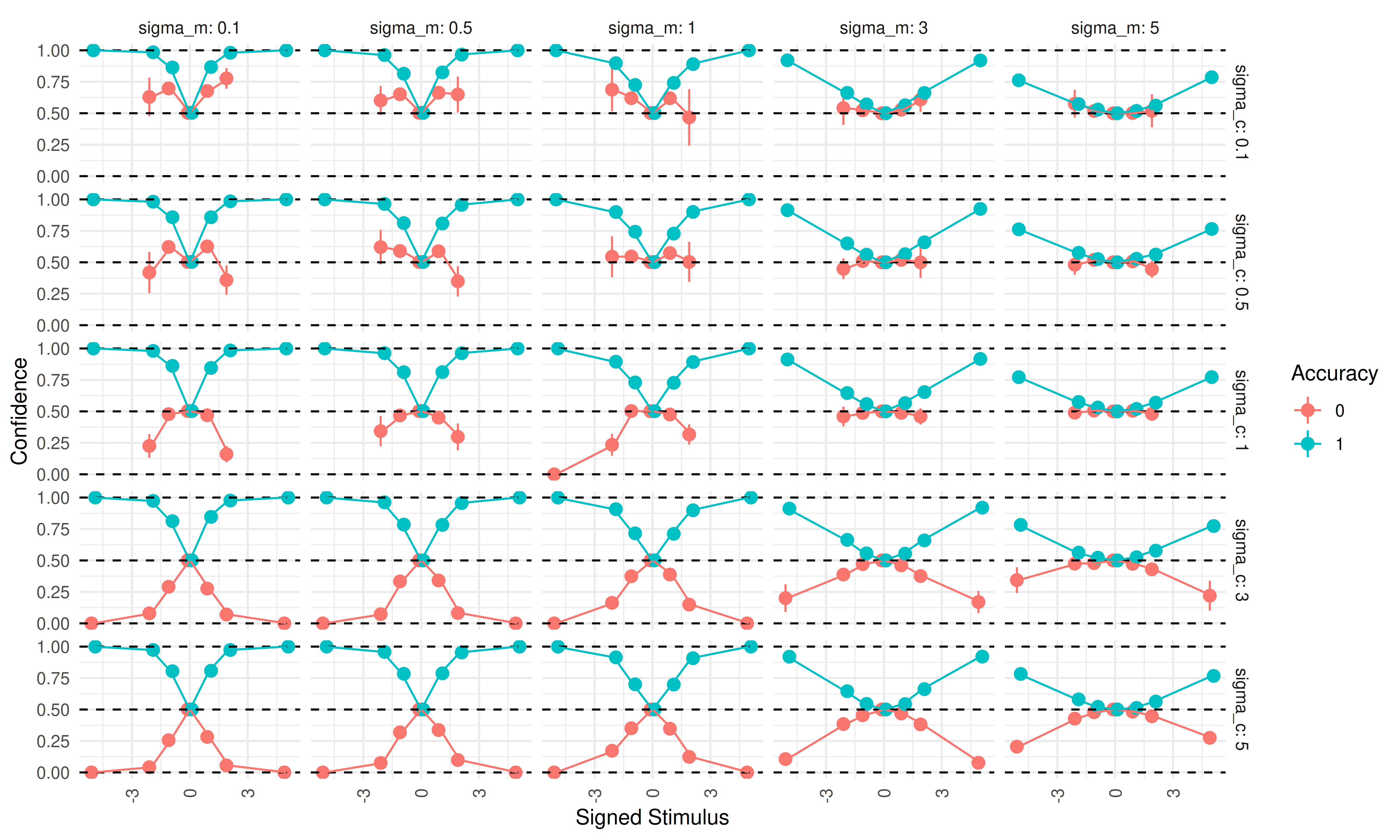
First, we fix \(\sigma_c = 1\) and examine how \(\sigma_e\) & \(\sigma_m\) change confidence ratings as a function of the signed stimulus intensity:
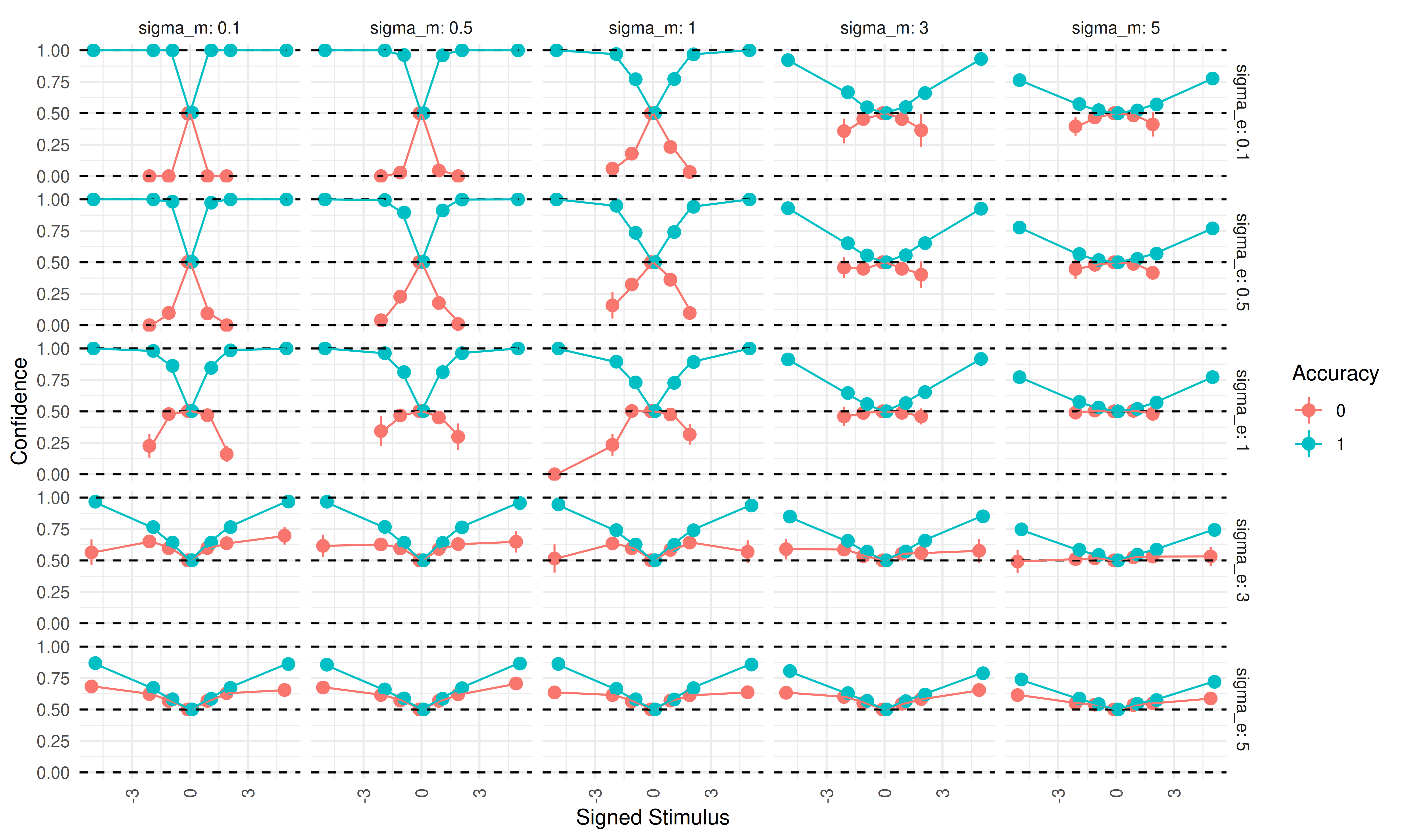
When confidence is plotted on the signed stimulus scale, a double-increase pattern emerges when \(\sigma_e\) is high (moving down the facets), and a folded-X pattern appears when \(\sigma_e\) is low (moving up the facets). As metacognitive noise (\(\sigma_m\)) increases (moving left to right), both confidence curves become increasingly flat (i.e., closer to 0.5) regardless of correctness.
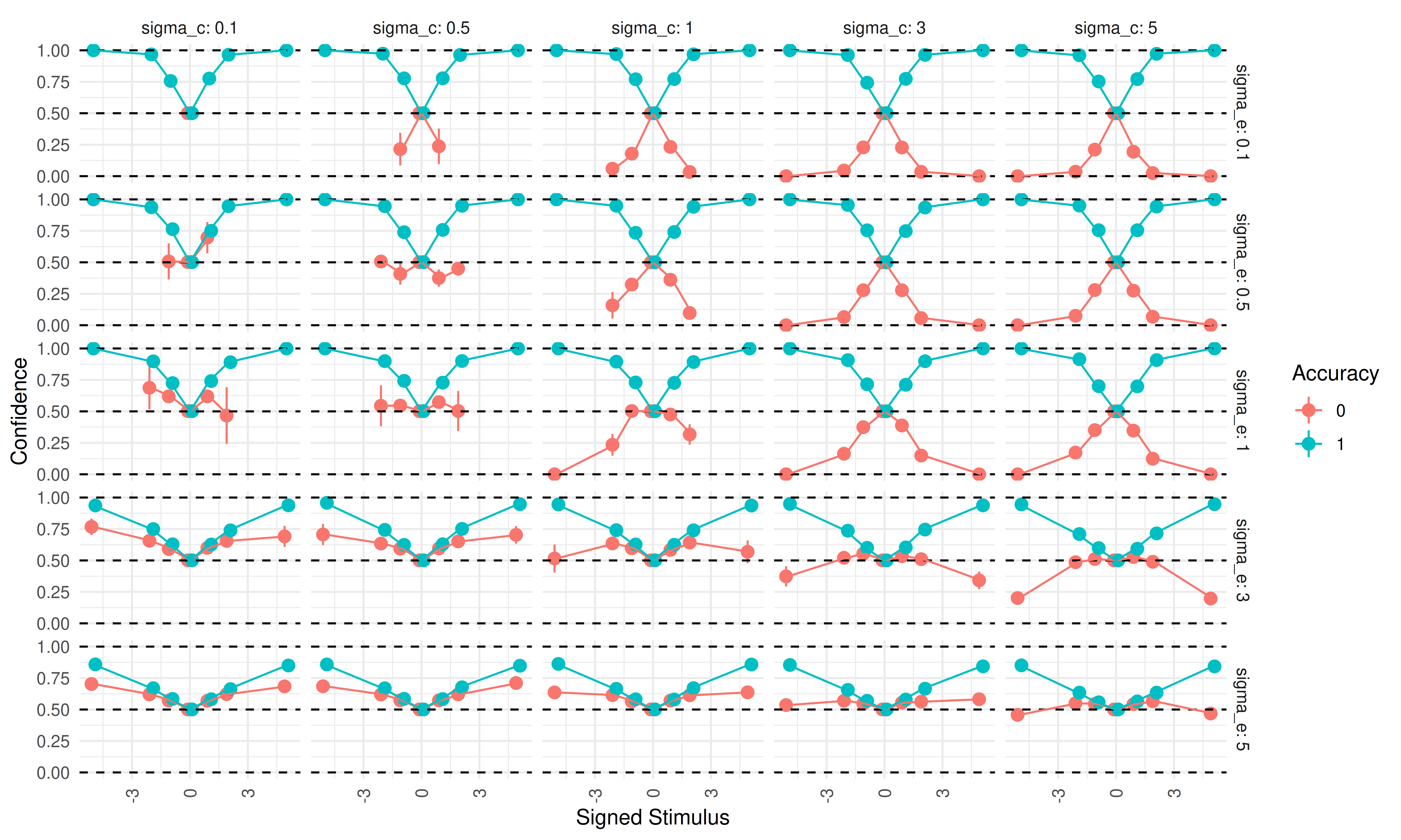
Next, we fix \(\sigma_e = 1\) and examine \(\sigma_c\) and \(\sigma_m\):
The pattern is similar to the previous plot. A high \(\sigma_c\) produces a folded-X, whereas lower values (especially below 1) produce a double-increase. As before, increasing metacognitive noise (\(\sigma_m\)) flattens both confidence curves toward 0.5 regardless of correctness.
Lastly, we plot simulated data for varying \(\sigma_c\) and \(\sigma_e\) with \(\sigma_m = 1\):
When \(\sigma_e = \sigma_c\) (the diagonal), it becomes difficult to distinguish folded-X from double-increase patterns, because incorrect trials cluster around 0.5 and show little dependence on stimulus intensity. Correct trials increase in confidence with stimulus intensity across all parameter combinations. In the upper triangle (where \(\sigma_c > \sigma_e\)), folded-X patterns emerge, whereas in the lower triangle (\(\sigma_c < \sigma_e\)), double-increase patterns emerge.
These simulations show that, in the current model, the double-increase and folded-X patterns arise from different ratios of encoding noise to choice variability. When choice variability is high relative to encoding noise, a folded-X pattern arises; when choice variability is low relative to encoding noise, a double-increase pattern arises. Metacognitive noise (\(\sigma_m\)) is agnostic to the accuracy of the rater and, when it increases, flattens the confidence curves regardless of correctness.
2.2.4 Fitting
We want to fit this model using full Bayesian inference with Stan’s NUTS sampler, treating the latent trial-by-trial evidence as parameters estimated jointly with subject-level noise parameters. In our pilot data, the model could be fit at the single-subject level with adequate sampler diagnostics. However, fitting it in a hierarchical framework (i.e., drawing subject-level parameters from group-level parameters) produced sampling issues. Because the current project uses a sequential sampling paradigm, a robust and efficient model is necessary. We therefore develop a heuristic model that approximates the model described above without requiring estimation of trial-by-trial evidence.
2.2.5 The Heuristic model
The computational complexity of the above model, especially in hierarchical settings, motivates a simpler heuristic approximation. The key challenge is that confidence requires trial-specific evidence \(r_i\), which cannot be marginalized analytically because the random variable is inside the inverse logit function.
The inverse logit function and the cumulative normal distribution are in practice nearly indistinguishable up to a scaling constant, i.e., \(g(\cdot) \approx \Phi(\cdot / 1.7)\), as shown below:
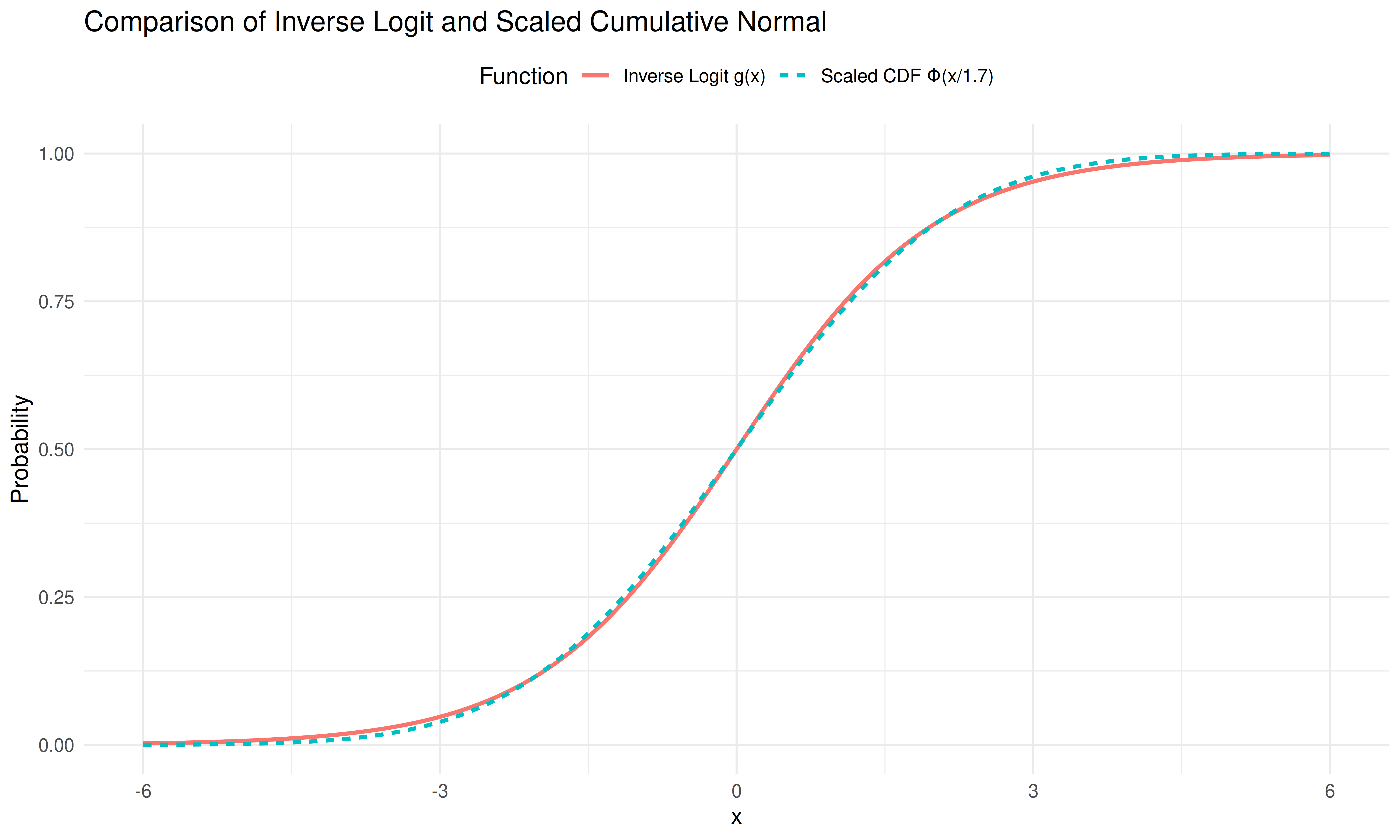
Using this approximation, it is possible to marginalize out the trial-by-trial evidence and arrive at a computationally less expensive model (and a closed-form equation for the expectation of confidence) that uses the same parameters.
With this approximation we go from equation (2) to the following:
\[ P(\text{correct} \mid r_i, a, X_i) = \begin{cases}\Phi\left(\frac{C \cdot r_i \cdot X_i}{\sigma_e^2 + \sigma_m^2}\right) & \text{if } a = 1 \\ 1 - \Phi\left(\frac{C \cdot r_i \cdot X_i}{\sigma_e^2 + \sigma_m^2}\right) & \text{if } a = -1\end{cases} \tag{3} \]
Where \(C = \frac{2}{1.7}\).
Focusing on the case where the choice is \(a = 1\):
\[ \Phi\left(\frac{C \cdot r_i \cdot X_i}{\sigma_e^2 + \sigma_m^2}\right) \]
We want to marginalize over \(r_i\), i.e. calculate the expectation of above equation, across \(r_i\). This can be done using the general formula for the expectation of a random continuous variable.
\[ \mathbb{E(X)} = \int_{-\infty}^\infty x \ p(x) dx \]
Substituting variables, with \(b = \frac{CX_i}{\sigma_e^2 + \sigma_m^2}\)
\[ \int_{-\infty}^\infty \Phi(b \cdot r_i) \ p(r_i) dr_i \]
with \(r_i \sim \mathcal{N}(\mu,\sigma)\)
This integral can be shown to have the solution:
\[ \Phi \left(\frac{\mu \cdot b}{\sqrt{1+\sigma^2 \cdot b^2}}\right) \]
Given that \(r_i \sim \mathcal{N}(X_iD_i - \beta, \sqrt{\sigma_m^2+\sigma_e^2})\), we get:
\[ \Phi \left(\frac{\mathbb{E}(r_i) \cdot b}{\sqrt{1+(\sigma_e^2+\sigma_m^2) \cdot b^2}}\right) \]
We write the expectation of \(r_i\), rather than the distributional mean of \(r_i\) i.e., \(X_iD_i - \beta\), because this expectation will be conditional on the choice (recall we are considering \(a_i = 1\)).
Expanding and simplifying, we obtain:
\[ \Phi\left(\frac{\mathbb{E}(r_i) \cdot CX_i}{ \sigma_e^2 + \sigma_m^2} \cdot\frac{1} {\sqrt{1 + \frac{C^2X^2_i}{\sigma_e^2+\sigma_m^2}}}\right) \]
This equation gives the probability of being correct when the choice is 1. However, because the rater knows the actor’s choice and the rater’s evidence is a noisy readout of the evidence used to generate that choice, observing the choice provides additional information about the underlying evidence. Mathematically, if the rater uses all available information, the expectation of the evidence must be conditional on the actor’s choice.
Equation (3) therefore becomes:
\[ P(\text{correct} \mid a, X_i) = \begin{cases} \Phi\left(\frac{\mathbb{E}(r_i \mid a = 1) \cdot CX_i}{\sigma_e^2 + \sigma_m^2} \cdot \frac{1}{\sqrt{1 + \frac{C^2X^2_i}{\sigma_e^2+\sigma_m^2}}}\right) & \text{if } a = 1 \\ 1 - \Phi\left(\frac{\mathbb{E}(r_i \mid a = -1) \cdot CX_i}{\sigma_e^2 + \sigma_m^2} \cdot \frac{1}{\sqrt{1 + \frac{C^2X^2_i}{\sigma_e^2+\sigma_m^2}}}\right) & \text{if } a = -1 \end{cases} \tag{4} \]
It can be shown that this conditional expectation equals the following equation (for a full derivation see below):
Click to expand: Calculating conditional expectations.
The goal here is to derive the two expectations of \(r_i\) given the choice i.e. \(\mathbb{E}(r_i \mid a_i = 1)\) and \(\mathbb{E}(r_i \mid a_i = -1)\)
To derive these expectations, we need to account for the fact that the choice \(a_i\) depends on the relationship between the evidence \(e_i\) and the criterion \(c_i\), and given that \(r_i\) is a noisy readout of \(e_i\) there is a dependency structure.
We have the following relationships:
- Evidence: \(e_i \sim \mathcal{N}(X_iD_i - \beta, \sigma_e)\)
- Criterion: \(c_i \sim \mathcal{N}(0, \sigma_c)\)
- Metacognitive evidence: \(r_i = e_i + \epsilon_m\) where \(\epsilon_m \sim \mathcal{N}(0, \sigma_m)\)
- Choice: \(a_i = 1\) if \(e_i > c_i\), otherwise \(a_i = -1\)
we can treat the difference distribution \(e_i - c_i\) as a joint bivariate normal distribution with \(r_i\) and calculate the expectation of \(r_i\) given that the \(e_i - c_i\) random variable is above 0 (or equivalently that the choice was 1).
The difference \(e_i - c_i\) follows a Gaussian distribution, as both random variables are Gaussian.
\[ (e_i - c_i) \sim \mathcal{N}(X_iD_i - \beta, \sqrt{\sigma_e^2 + \sigma_c^2}) \] The joint bivariate normal distribution becomes:
\[ \begin{bmatrix} e_i - c_i \\ r_i \end{bmatrix} \sim \mathcal{N}\left( \begin{bmatrix} X_iD_i - \beta \\ X_iD_i - \beta \end{bmatrix}, \begin{bmatrix} \sigma_e^2 + \sigma_c^2 & \sigma_e^2 \\ \sigma_e^2 & \sigma_e^2 + \sigma_m^2 \end{bmatrix} \right) \]
Intuitively this bivariate normal distribution can be argued for by realizing that both distributions of \(e_i - c_i\) and \(r_i\) share \(e_i\), with the same mean but are otherwise independent.
The key mathematical insight is that the covariance between \(e_i-c_i\) and \(r_i\) is \(\sigma_e^2\) and not zero.
Writing the full covariance and expanding it using this we get:
\[ \text{Cov}(e_i-c_i, r_i) = \text{Cov}(e_i-c_i, e_i + \epsilon_m) \] \[ \text{Cov}(e_i-c_i, r_i) = \text{Cov}(e_i,e_i) + \text{Cov}(e_i, \epsilon_m) - \text{Cov}(c_i,e_i) - \text{Cov}(c_i, \epsilon_m)= \text{Cov}(e_i,e_i) = \text{Var}(e) =\sigma_e^2 \] As \(e_i\) and \(\epsilon_m\) and also \(c_i\) are independent, these covariances are 0:
\[ \text{Cov}(e_i-c_i, r_i) = \text{Cov}(e_i,e_i) = \text{Var}(e) =\sigma_e^2 \]
This shared variance structure means that \(e_i-c_i\) and \(r_i\) are correlated with correlation coefficient.
\[ \rho = \frac{\sigma_e^2}{\sqrt{(\sigma_e^2 + \sigma_c^2)} \cdot \sqrt{(\sigma_e^2 + \sigma_m^2)}} \tag{5} \]
2.2.5.1 Truncated normal distributions
To proceed, we need a general result from probability theory. Suppose we have two jointly normal random variables:
\[ \begin{pmatrix} Z \\ Y \end{pmatrix} \sim \mathcal{N}\left(\begin{pmatrix} \mu_Z \\ \mu_Y \end{pmatrix}, \begin{pmatrix} \sigma_Z^2 & \rho\sigma_Y\sigma_Z \\ \rho\sigma_Y\sigma_Z & \sigma_Y^2 \end{pmatrix}\right) \] It can be shown that the expectation of Y given Z>0 is:
\[ \mathbb{E}(Y \mid Z > 0) = \mu_Y + \rho\cdot \sigma_Y\frac{\phi(z_z)}{\Phi(z_z)} \]
With \(z_Z = \frac{\mu_Z}{\sigma_Z}\)
The key idea is that we want to find \(\mathbb{E}(Y \mid Z > 0)\), the expected value of \(Y\) conditional on \(Z\) being positive (i.e. the choice was 1).
From standard bivariate normal theory, the conditional distribution of \(Y\) given \(Z = z\) is:
\[ Y \mid Z = z \sim \mathcal{N}\left(\mu_Y + \rho\cdot\frac{\sigma_Y}{\sigma_Z}(z - \mu_Z), \sigma_Y^2(1-\rho^2)\right) \]
(see https://uregina.ca/~kozdron/Teaching/Regina/351Fall15/Handouts/351lect24.pdf)
So if we take the expectation of this conditional distribution \(\mathbb{E}(Y \mid Z = z) = \mu_Y + \rho\cdot \frac{\sigma_Y}{\sigma_Z}(z - \mu_Z)\) (instead of conditioning on Z we want the expectation of Y when Z > 0, i.e. the expectation of \(r_i\) when the choice was 1)
\[ \mathbb{E}(Y \mid Z > 0) = \mu_Y + \rho\cdot \frac{\sigma_Y}{\sigma_Z}(\mathbb{E}(Z | Z >0) - \mu_Z) \]
From here we have that the expectation of a truncated normal distribution can be written as: https://en.wikipedia.org/wiki/Truncated_normal_distribution
\[ \mathbb{E}(Z | Z > a) = \mu_Z + \sigma_Z \frac{\phi(\frac{a-\mu_Z}{\sigma_Z})}{1-\Phi(\frac{a-\mu_Z}{\sigma_Z})} \]
which in this case reduces to when a = 0
\[ \mathbb{E}(Z | Z > 0) = \mu_Z + \sigma_Z \frac{\phi(-z_z)}{1-\Phi(-z_z)} \]
given that \(-Z_z = \frac{-\mu_Z}{\sigma_Z}\)
Now using that the pdf of the Gaussian is symmetrical i.e. \(\phi(x) = \phi(-x)\) and also that \(1-\Phi(-x) = \Phi(x)\)
\[ \mathbb{E}(Z | Z > 0) = \mu_Z + \sigma_Z \frac{\phi(z_z)}{\Phi(z_z)} \]
Finally inserting this into the equation:
\[ \mathbb{E}(Y \mid Z > 0) = \mu_Y + \rho\cdot \frac{\sigma_Y}{\sigma_Z}(\mathbb{E}(Z | Z >0) - \mu_Z) \] we get:
\[ \mathbb{E}(Y \mid Z > 0) = \mu_Y + \rho\cdot \frac{\sigma_Y}{\sigma_Z}(\mu_Z + \sigma_Z \frac{\phi(z_z)}{\Phi(z_z)} - \mu_Z) \]
which reduces to:
\[ \mathbb{E}(Y \mid Z > 0) = \mu_Y + \rho\cdot \sigma_Y\frac{\phi(z_z)}{\Phi(z_z)} \]
Now replacing Y with \(r_i\) and Z with \(e_i - c_i\) we get:
\[ \mathbb{E}(r_i \mid (e_i-c_i) > 0) = (X_iD_i - \beta) + \rho \cdot \sqrt{\sigma_e^2 + \sigma_m^2} \cdot \frac{\phi(z_z)}{\Phi(z_z)} \]
With \(z_z = \frac{X_iD_i - \beta}{\sqrt{\sigma_e^2 + \sigma_c^2}}\)
It can then easily be shown using the same steps that when the action is -1 i.e. \((e_i-c_i) < 0\) this becomes:
\[ \mathbb{E}(r_i \mid (e_i-c_i) < 0) = (X_iD_i - \beta) - \rho \cdot \sqrt{\sigma_e^2 + \sigma_m^2} \cdot \frac{\phi(-z_z)}{\Phi(-z_z)} \]
we might define \(\lambda(x) = \frac{\phi(x)}{\Phi(x)}\), which is the inverse Mills ratio.
\[ \mathbb{E}(r_i \mid a = 1) = (X_iD_i - \beta) + \rho \cdot \sqrt{\sigma_e^2 + \sigma_m^2} \cdot \lambda\left(\frac{X_iD_i - \beta}{\sqrt{\sigma_e^2 + \sigma_c^2}}\right) \]
For \(a = -1\):
\[ \mathbb{E}(r_i \mid a = -1) = (X_iD_i - \beta) - \rho \cdot \sqrt{\sigma_e^2 + \sigma_m^2} \cdot \lambda\left(-\frac{X_iD_i - \beta}{\sqrt{\sigma_e^2 + \sigma_c^2}}\right) \]
Here \(\lambda(x) = \frac{\phi(x)}{\Phi(x)}\), and \(\rho = \frac{\sigma_e^2}{\sqrt{(\sigma_e^2 + \sigma_c^2)} \cdot \sqrt{(\sigma_e^2 + \sigma_m^2)}}\).
2.2.6 Final confidence model
Substituting these conditional expectations back into equation (4) and simplifying gives:
\[ P(correct \mid a = 1, X_i, D_i) = \Phi\left(\left[\frac{(CX_i^2D_i - C\beta X_i)}{\sigma_e^2 + \sigma_m^2} + \rho \cdot \frac{ \lambda\left(\frac{X_iD_i - \beta}{\sqrt{\sigma_e^2 + \sigma_c^2}}\right)CX_i}{\sqrt{\sigma_e^2 + \sigma_m^2} }\right] \cdot\frac{1} {\sqrt{1 + \frac{C^2X^2_i}{\sigma_e^2+\sigma_m^2}}}\right) \]
This gives a fully marginalized model for confidence ratings (for choices of \(a = 1\)) that depends only on the parameters \(\Theta_1 = (\beta, \sigma_e, \sigma_c, \sigma_m)\) and the observed data (choices \(a_i\), stimuli \(X_i\), and true states \(D_i\)), without requiring trial-by-trial estimation of the latent evidence variables \(e_i\) and \(r_i\).
Before interpreting this equation, we return to a key assumption outlined just after equation (2): computing the subjective probability of being correct requires that the participant has access to the stimulus intensity. Below, we highlight the two \(X_i\) terms in the equation that depend on this assumption:
\[ P(\text{correct} \mid a = 1, X_i, D_i) = \Phi\left(\frac{\left[(X_iD_i - \beta) + \rho \cdot \sqrt{\sigma_e^2 + \sigma_m^2} \cdot \lambda\left(\frac{X_iD_i - \beta}{\sqrt{\sigma_e^2 + \sigma_c^2}}\right)\right] \cdot C \mathbf{X_i}}{ \sigma_e^2 + \sigma_m^2} \cdot\frac{1} {\sqrt{1 + \frac{C^2\mathbf{X^2_i}}{\sigma_e^2+\sigma_m^2}}}\right) \]
These two stimulus intensity terms (shown in bold), especially the first (which does not arise from the marginalization), ensure that at intensity 0 the predicted confidence is always 0.5. This is a strong assumption: it requires the agent to have access to the objective stimulus strength, and the assumption is also inconsistent with the empirical observation (highlighted in Part 1) that the lowest confidence rating shifts with bias. If confidence ratings are treated as noisy, biased subjective probabilities of being correct, the formulation above becomes problematic because of its reliance on an objective anchor at \(X_i = 0\). Based on these considerations, supported by empirical validation on our pilot data below, we believe this particular stimulus intensity term, which rests on an unjustified assumption, needs to be addressed.
One possible solution is to assume that the agent has a noisy readout of stimulus strength, \(\hat{X} \sim p(\hat{x}|\theta,c)\). The difficulty with this formulation is defining the probability distribution of the internal stimulus intensity. This distribution must be positively bounded (\(\hat{X} > 0\)), which introduces an arbitrary distributional choice and, more importantly, makes it nontrivial to marginalize the trial-by-trial readout. An alternative approach would be to replace the stimulus intensity with a participant-specific constant, serving as a placeholder for idiosyncratic differences in how participants use stimulus intensity information beyond what they should have access to.
Instead, we assume that agents do not have access to this stimulus intensity and fix it to 1. This approach circumvents the computational difficulties mentioned above while remaining consistent with what the agent is assumed to have access to. It also allows the model to accommodate the empirical observation that the confidence curve follows the psychometric function of the binary choices. Below, we show that in our pilot data, the two models (fixing this stimulus intensity to 1 versus letting it vary with the true stimulus intensity) have equivalent approximate leave-one-out cross-validation performance.
The final equations becomes:
\[ P(\text{correct} \mid a = 1, X_i, D_i) = \Phi\left(\left[\frac{(CX_iD_i - C\beta)}{\sigma_e^2 + \sigma_m^2} + \rho \cdot \frac{ \lambda\left(\frac{X_iD_i - \beta}{\sqrt{\sigma_e^2 + \sigma_c^2}}\right)C}{\sqrt{\sigma_e^2 + \sigma_m^2} }\right] \cdot\frac{1} {\sqrt{1 + \frac{C^2}{\sigma_e^2+\sigma_m^2}}}\right) \tag{7a} \]
which for \(a = -1\) becomes:
\[ P(\text{correct} \mid a = -1, X_i, D_i) = 1-\Phi\left(\left[\frac{(CX_iD_i - C\beta)}{\sigma_e^2 + \sigma_m^2} - \rho \cdot \frac{ \lambda\left(-\frac{X_iD_i - \beta}{\sqrt{\sigma_e^2 + \sigma_c^2}}\right)C}{\sqrt{\sigma_e^2 + \sigma_m^2} }\right] \cdot\frac{1} {\sqrt{1 + \frac{C^2}{\sigma_e^2+\sigma_m^2}}}\right) \tag{7b} \]
with:
\[ \begin{aligned} \lambda(x) &= \frac{\phi(x)}{\Phi(x)} \\ C &= \frac{2}{1.7} \end{aligned} \]
In the above formula it is noteworthy that the terms inside the cumulative normal distribution function have clear interpretations.
First, the common factor is a correction for marginalization:
\[ K_i = \frac{1}{\sqrt{1 + \frac{C^2}{\sigma_e^2+\sigma_m^2}}} \]
The two remaining terms have direct cognitive interpretations. Returning to equation (3) (now with \(X_i = 1\)), the first term from equations (7a/7b) is the expectation of the log-likelihood ratio (the argument inside \(\Phi(\cdot)\)). It can be interpreted as the prior belief about being correct based purely on the stimulus, before any information about the action is taken into account:
\[ I_i = \mathbb{E}\left(\frac{C \cdot r_i}{\sigma_e^2 + \sigma_m^2}\right) = \frac{C(X_iD_i - \beta)}{\sigma_e^2 + \sigma_m^2} \]
The second term updates this prior using the information carried by the action via the efference copy:
\[ S_i = \pm\rho \cdot \frac{\lambda\left(\pm\frac{X_iD_i - \beta}{\sqrt{\sigma_e^2 + \sigma_c^2}}\right)C}{\sqrt{\sigma_e^2 + \sigma_m^2}} \]
This term functions as an internal action prediction error: it reflects the discrepancy between the action the evidence predicted and the action actually executed, as observed through the noisy efference copy channel. Its magnitude is governed by the inverse Mills ratio \(\lambda(\cdot)\), which is large when the action was surprising given the evidence (i.e., errors at high stimulus intensity) and near zero when the action was expected (i.e., correct responses at high stimulus intensity). Confidence in probit space is therefore the sum of a prior and a prediction error, scaled by the correction factor:
\[ \Phi^{-1}(\mu_{c_i}) = (I_i + S_i) \cdot K_i \]
This is analogous to a reinforcement learning rule where a prior value estimate is corrected by a prediction error, but here no external feedback is necessary; the efference copy itself serves as the internal reference signal. The addition of action information to the confidence computation was proposed in the second-order rater model of Fleming and Daw (2017), with empirical support from reanalysis of behavioral data. The present formulation makes the mechanism explicit: the efference copy supplies the prediction error.
For completeness, we show the magnitude of these two terms as a function of signed stimulus intensity. For a range of stimulus intensities \(U(0.05,1)\), we show how both \(I_i\) and \(S_i\) vary with choice correctness.
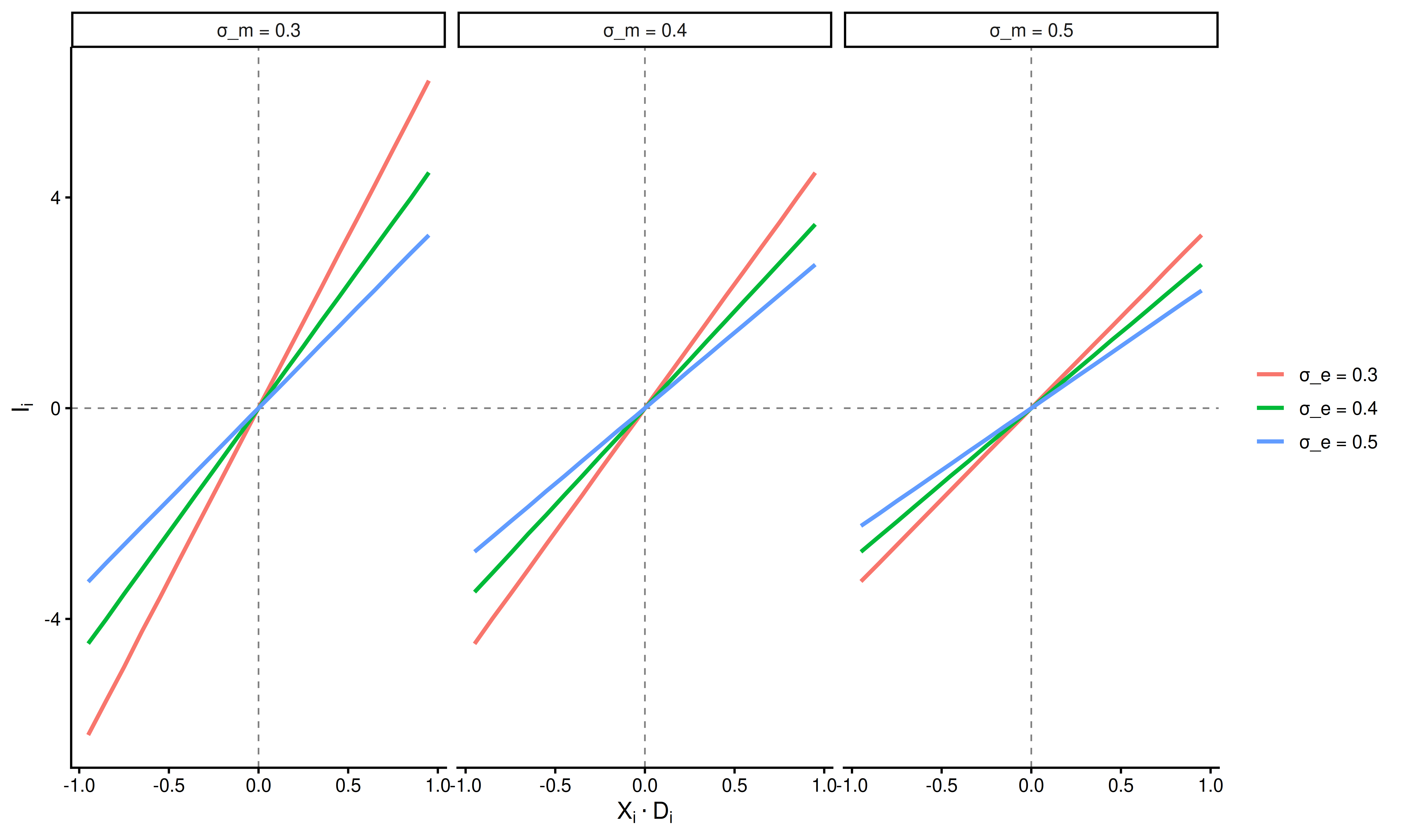
Here \(\sigma_m\) and \(\sigma_e\) have qualitatively the same effect on \(I_i\), both reduce the strength of the relationship between signed stimulus intensity and average evidence in favor of the true state.
Next, we examine how the parameters influence the second term \(S_i\). First, we plot varying levels of \(\sigma_m\) with \(\sigma_e = 0.5\) and \(\sigma_c = 0.5\)
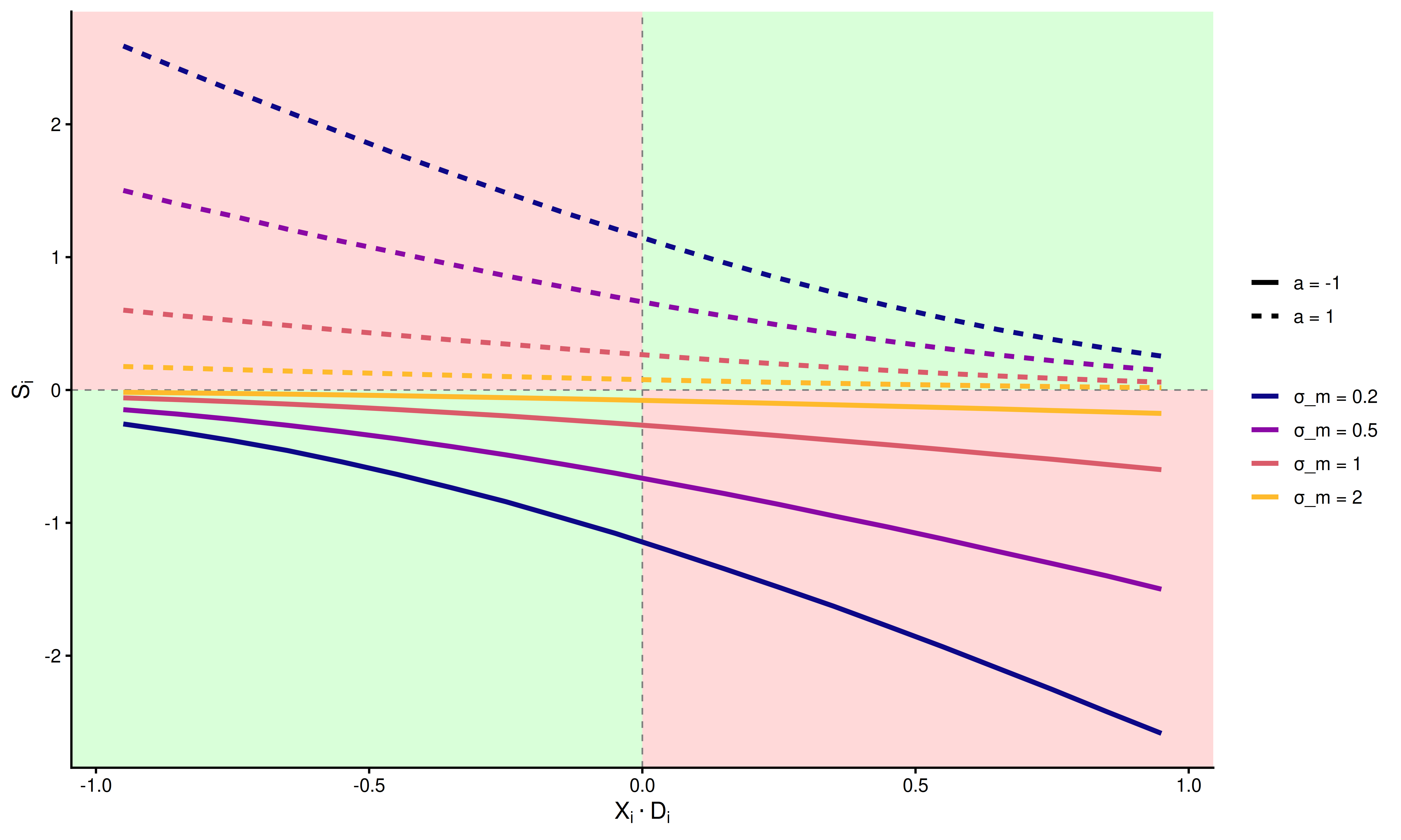
In the above plot, each quadrant corresponds to a different state of the decision process. Green quadrants indicate correct responses; red quadrants indicate errors. Line color represents different levels of metacognitive noise \(\sigma_m\). The magnitude of \(S_i\) is uniformly attenuated as \(\sigma_m\) increases.
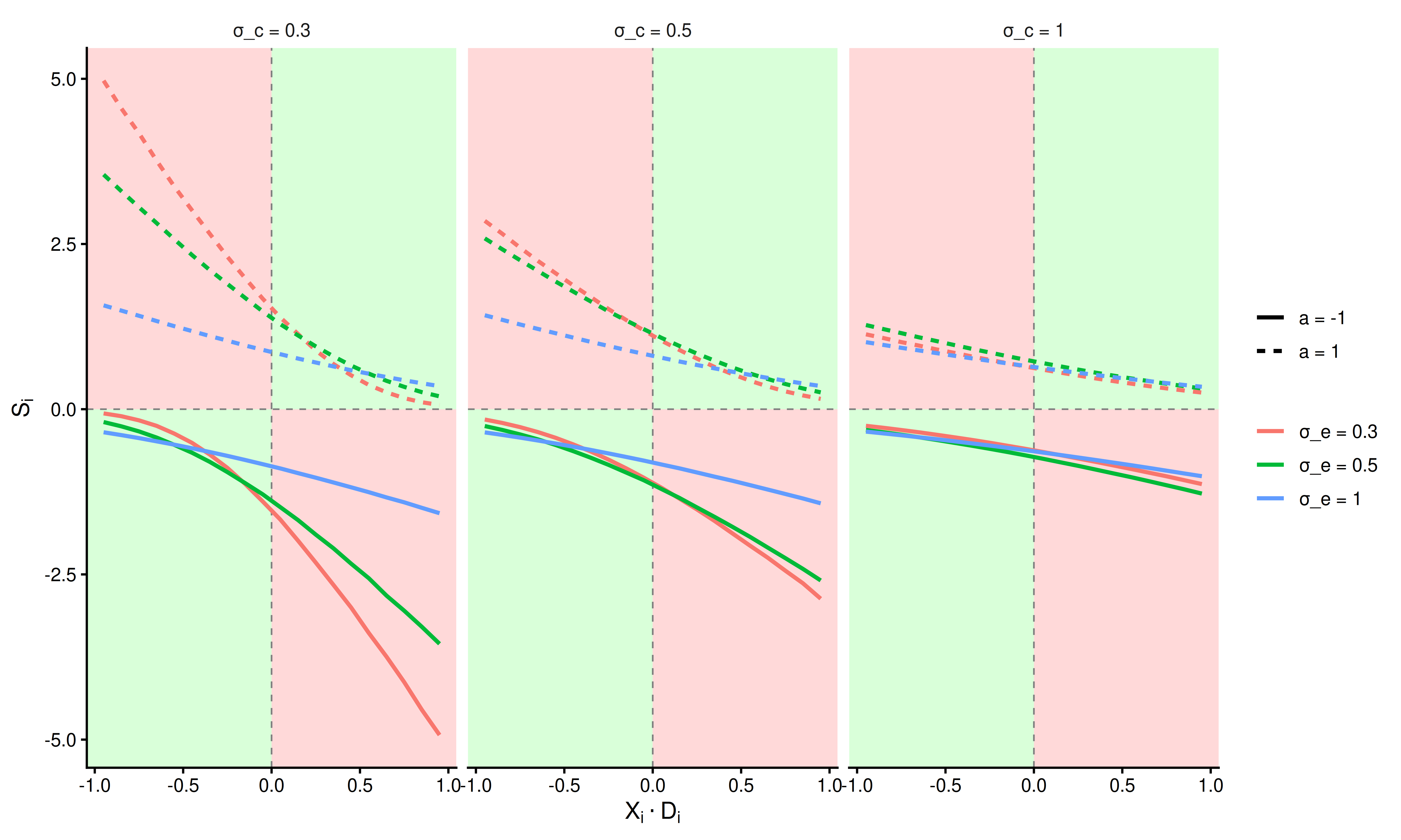
The same quadrant structure applies. The plot shows that increasing either \(\sigma_e\) or \(\sigma_c\) reduces the magnitude of \(S_i\).
To summarize, confidence in this model is the sum of a stimulus-based prior \(I_i\) and an action-based prediction error \(S_i\), scaled by the marginalization factor \(K_i\). The prediction error is largest for incorrect responses at high stimulus intensity and smallest for correct responses at high stimulus intensity. This pattern has implications for how physiological responses, particularly pupil dilation, may track the decision process.
2.2.6.1 Additional parameters
We introduce 5 additional parameters. \(\Theta_2 = (\kappa_c, \gamma, \mu_{\beta}, c_0,c_1)\).
\(\gamma\) is the lapse rate on the binary choices, a stimulus independent factor that shifts the asymptote of the psychometric function away from certainty i.e., the asymptotes become \(\gamma\) and \(1-\gamma\).
\(\mu_{\beta}\) is a metacognitive bias parameter, serving as an independent vertical shift of confidence ratings.
\(\kappa_c\) is the precision of the ordered beta likelihood.
\(c_0\),\(c_1\) are the two cutpoints for the ordered beta likelihood. These two parameters help generalize the beta-distribution to outcomes that include 0 and 1 ratings.
See (Kubinec 2023) for the ordered beta likelihood.
The complete set of parameters for the model is:
\[ \begin{aligned} \Theta_s &= \begin{bmatrix} \beta_s \\ \sigma_{e_s} \\ \sigma_{c_s} \\ \sigma_{m_s} \\ \mu_{\beta_s} \\ \kappa_{c_s} \\ \gamma_s \end{bmatrix} \sim \mathcal{N}(\mu_{\Theta},\Sigma_{\Theta}) \\ \text{where } & \beta_s \in [-1,1], \sigma_{e_s} >0, \sigma_{c_s} >0, \sigma_{m_s} > 0, \\ & \mu_{\beta_s} \in \mathbb{R}, \kappa_{c_s} > 0, \gamma_s \in [0,0.5] \\ & (c_{1_s} , c_{0_s}) \sim \delta([1,10,1]) \end{aligned} \]
In this formulation, \(\mathcal{N}\) denotes a multivariate normal distribution with mean and covariance. All parameter constraints are enforced through transformations: positively constrained parameters are exponentiated, and bounded parameters are transformed with the inverse logit function and scaled appropriately. The cutpoint constraints are imposed via a Dirichlet prior (\(\delta()\)). Note that cutpoints are sampled on a subject-by-subject basis.
The priors of the model are as follows:
\[ \begin{align*} \mu_{\beta} &\sim \mathcal{N}(0, 0.5) & \text{(group mean of threshold)} \\ \mu_{\sigma_{e_s}} &\sim \mathcal{N}(-2, 2) & \text{(group mean of encoding uncertainty)} \\ \mu_{\sigma_{c_s}} &\sim \mathcal{N}(-2, 2) & \text{(group mean of choice variability)} \\ \mu_{\sigma_{m_s}} &\sim \mathcal{N}(-2, 2) & \text{(group mean of meta uncertainty)} \\ \mu_{\beta_c} &\sim \mathcal{N}(0, 0.5) & \text{(group mean of meta bias)} \\ \mu_{\gamma_s} &\sim \mathcal{N}(2, 2) & \text{(group mean of lapse rate)} \\ \mu_{\kappa_c} &\sim \mathcal{N}(-4, 2) & \text{(group mean of confidence precision)} \\ \end{align*} \]
\[ \begin{align*} \tau_{\beta} &\sim \mathcal{N}(1, 1) & \text{(Between subject SD of threshold)} \\ \tau_{\sigma_{e_s}} &\sim \mathcal{N}(1, 1) & \text{(Between subject SD of encoding uncertainty)} \\ \tau_{\sigma_{c_s}} &\sim \mathcal{N}(1, 1) & \text{(Between subject SD of choice variability)} \\ \tau_{\sigma_{m_s}} &\sim \mathcal{N}(1, 1) & \text{(Between subject SD of meta uncertainty)} \\ \tau_{\beta_c} &\sim \mathcal{N}(1, 1) & \text{(Between subject SD of meta bias)} \\ \tau_{\gamma_s} &\sim \mathcal{N}(1, 1) & \text{(Between subject SD of lapse rate)} \\ \tau_{\kappa_c} &\sim \mathcal{N}(1, 1) & \text{(Between subject SD of confidence precision)} \\ \end{align*} \]
- \(\mathbf{R} \sim \mathrm{LKJ}(\eta = 2)\) (correlation matrix for the multivariate normal distribution.)
- \(z_{expo} \sim \mathcal{N}(0, 1)\) (participant deviations)
- \(c_0, c_{1}\): see Dirichlet prior in Stan code
The full model is
\[ \begin{aligned} P(a = 1) &= \Phi\left(\frac{D_i \cdot X_i- \beta_s}{\sqrt{\sigma_{e_s}^2 + \sigma_{c_s}^2}}\right) \\ \mu_{c_i} &= \begin{cases}\Phi\left((I_i-S_i)\cdot K_i\right) & \text{if } a_i = 1 \\ 1 - \Phi\left((I_i+S_i)\cdot K_i\right) & \text{if } a_i = -1\end{cases} \\ a_i &\sim \mathcal{bernoulli}(p(a_i = 1)) \\ Conf_i &\sim \mathcal{ord\beta}(\mu_{c_i},\kappa_{c_s},c_{0_s},c_{1_s}) \end{aligned} \]
with
\[ I_i = \frac{(CX_iD_i - C\beta)}{\sigma_{e_s}^2 + \sigma_{m_s}^2}, \quad S_i = -\rho_s \cdot \frac{ \lambda\left(-\frac{X_iD_i - \beta_s}{\sqrt{\sigma_{e_s}^2 + \sigma_{c_s}^2}}\right)C}{\sqrt{\sigma_{e_s}^2 + \sigma_{m_s}^2} }, \quad K_i = \frac{1} {\sqrt{1 + \frac{C^2}{\sigma_{e_s}^2+\sigma_{m_s}^2}}} \]
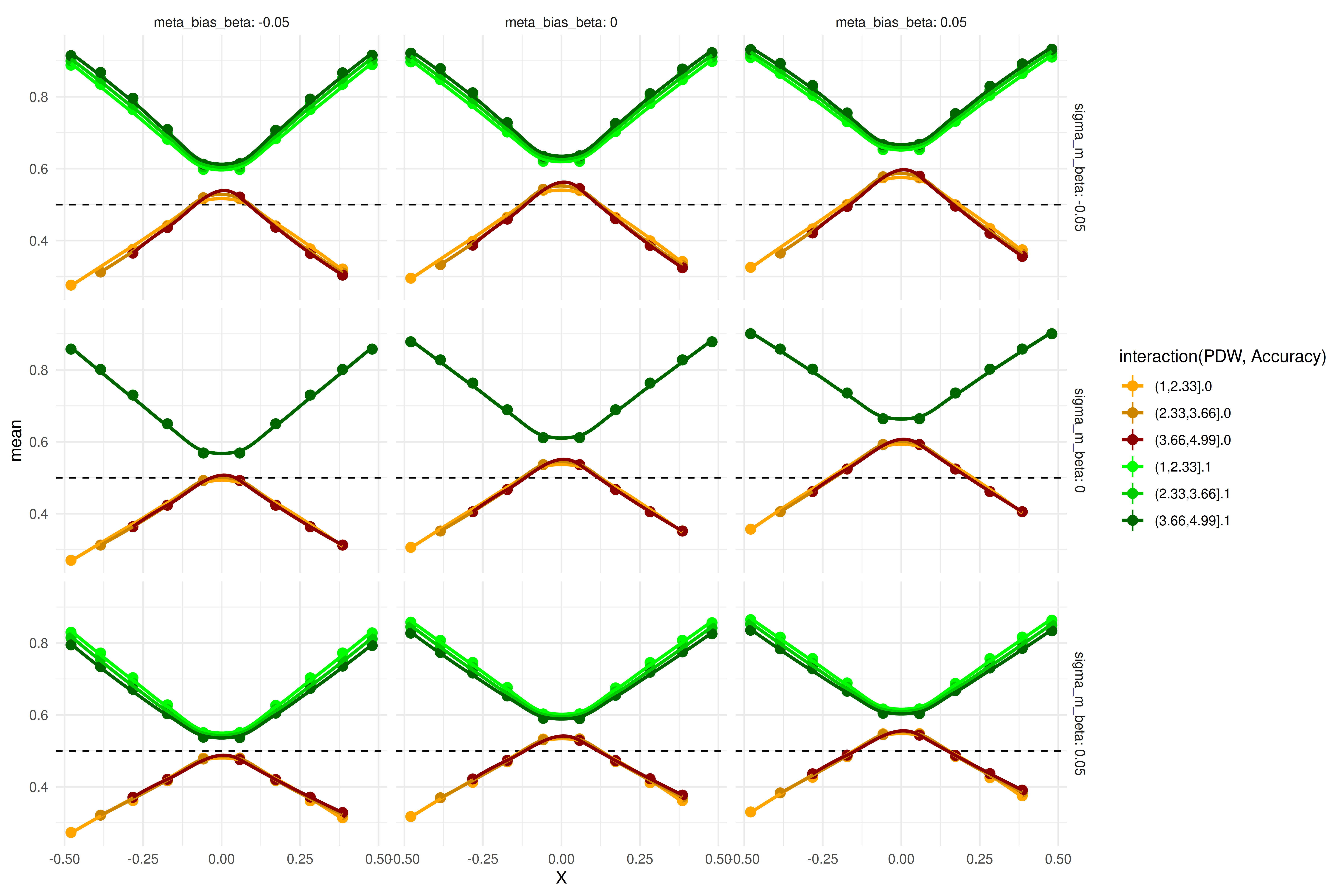
Next, we verify the marginalized heuristic model by simulating data from equation (2) (with \(X_i = 1\)), averaging across the signed stimulus axis, and displaying the predictions of the marginalized heuristic model for the same parameter values (\(\Theta_1\)).
In the first validation step, we simulate from different combinations of noise parameters (shown as facets).
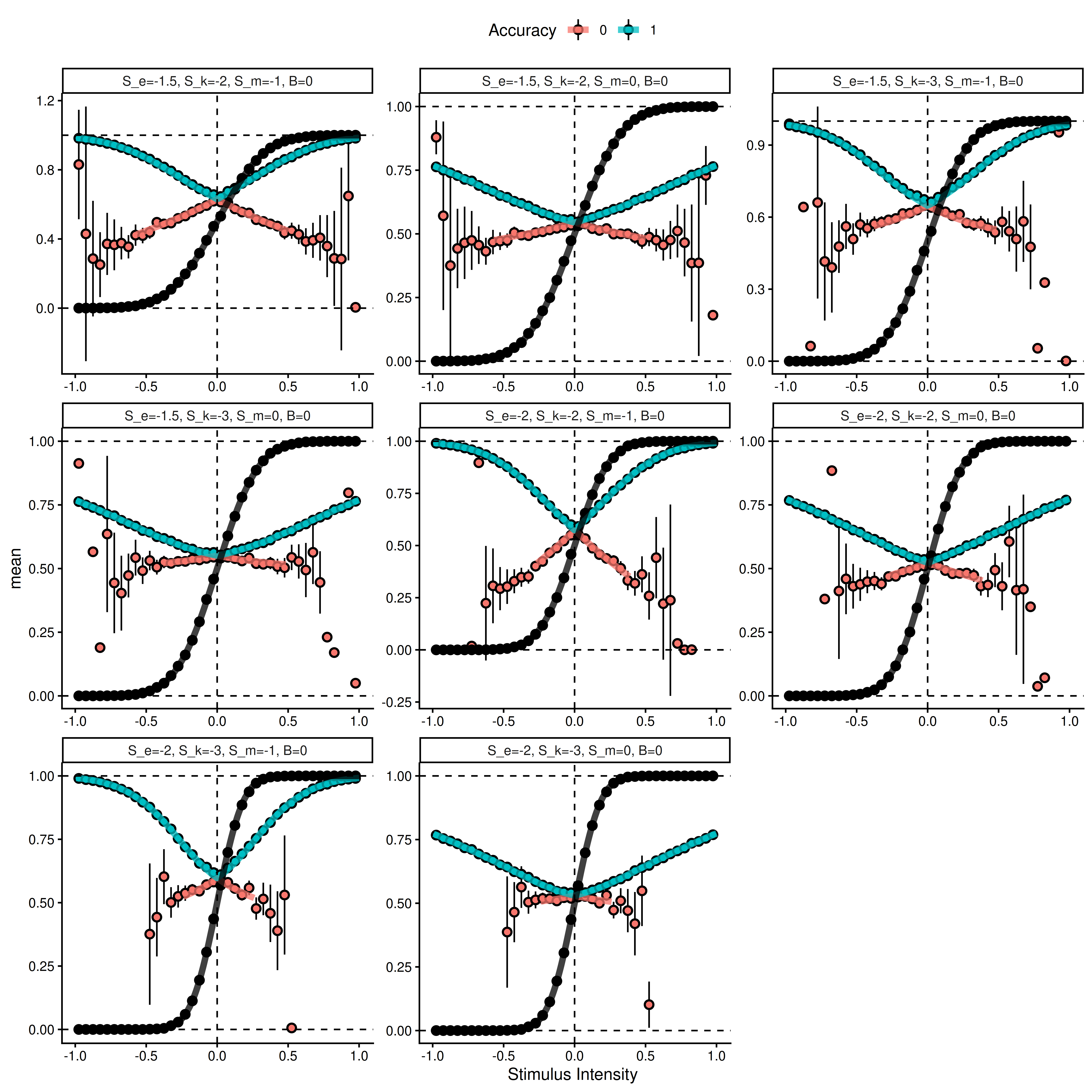
The above plot shows results from averaging 5^{5} simulated trials from equation (2) for each bin of the signed stimulus intensity scale (dots are means with approximate 95% intervals). The thick solid lines represent the marginalized heuristic model predictions.
Next, we simulate using fixed noise parameters and vary the bias \(\beta\). Note that here we display the action rather than the accuracy of the choice.
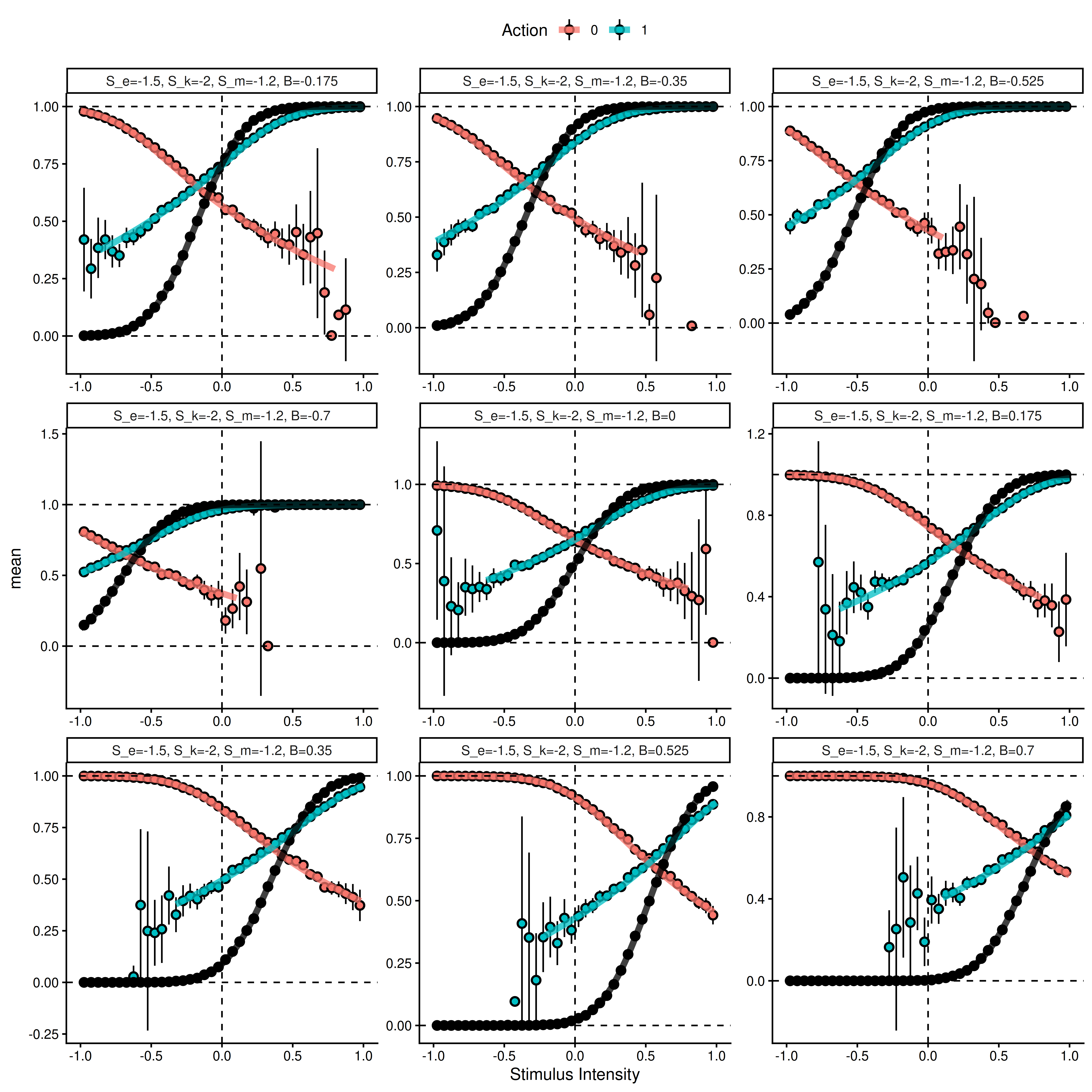
The above plot shows results from averaging 5^{5} simulated trials from equation (2) for each bin of the signed stimulus intensity scale (dots are means with approximate 95% intervals). The thick solid lines represent the marginalized heuristic model predictions.
2.2.7 Model for the current experiment.
In the current experiment, participants are presented with a random dot kinematogram on each trial and asked to choose which direction the majority of dots are moving. After an experimental delay (post-decisional response window), participants give a confidence rating. We aim to test whether this post-decisional response window changes the metacognitive noise and metacognitive bias parameters of the above model. This is implemented as follows:
\[ \sigma_{m_t} = \sigma_{m_s} + \Delta{\sigma_{m_s}} \cdot PDW_t\\ \mu_{\beta_t} = \mu_{\beta_s} + \Delta{\mu_{\beta_s}} \cdot PDW_t \]
The subject-level changes due to the post-decisional window (PDW) are drawn from additional group-level parameters in the multivariate normal distribution described above. These group-level parameters are given the following priors:
$$ \[\begin{align*} \mu_{\Delta{\sigma_{m_s}}} &\sim \mathcal{N}(0, 0.5) & \text{(group mean of effect of PDW on meta uncertainty)} \\ \mu_{\Delta{\mu_{\beta_c}}} &\sim \mathcal{N}(0, 0.5) & \text{(group mean of effect of PDW on meta bias)} \\ \tau_{\Delta{\sigma_{m_s}}} &\sim \mathcal{N}(0, 0.5) & \text{(Between subject SD of effect of PDW on meta uncertainty)} \\ \tau_{\Delta{\mu_{\beta_c}}} &\sim \mathcal{N}(0, 0.5) & \text{(Between subject SD of effect of PDW on meta bias)} \\ \end{align*}\] $$
PDW denotes the post-decisional response window.
\({\Delta{\sigma_{m_s}}}\) and \(\Delta{\mu_{\beta_c}}\) denote the change in metacognitive noise and metacognitive bias due to PDW, respectively.
Next, we investigate how this model, with metacognitive noise and metacognitive bias varying by PDW, fits our pilot data. The first step is model comparison using approximate leave-one-out cross-validation between the model assuming the rater has access to the objective stimulus intensity and the reduced model where \(X_i = 1\).
2.2.8 Model comparison
As a sanity check on the \(X_i = 1\) assumption, we fitted both hierarchical models to our pilot data and computed approximate leave-one-out cross-validation. The two models were virtually indistinguishable, with the difference in expected log predictive density being -1.58 \(\pm\) 9.9. A difference below \(-4\) or more than two standard errors from zero is generally considered evidence for one model over the other (REF); thus, at least in our pilot data, there is no difference in predictive performance. To further examine the distinction, we plot all pairwise parameter estimates below together with the identity line.
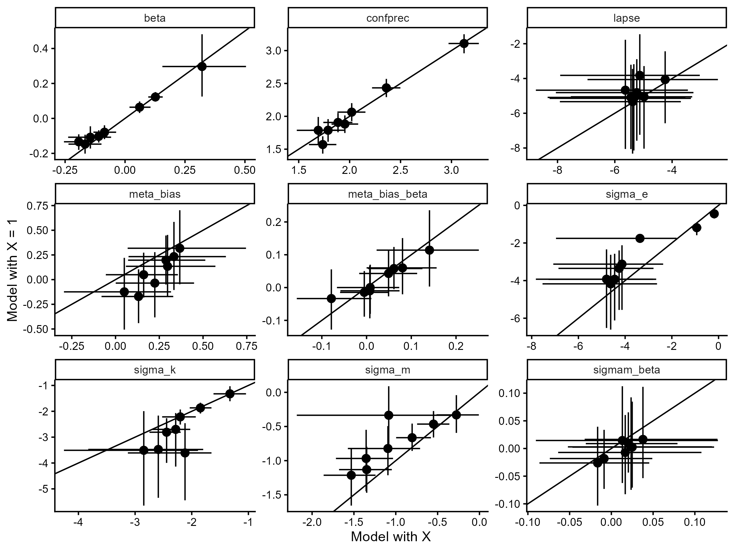
The two models align well in their subject-level parameter estimates, further justifying this theoretically motivated simplification.
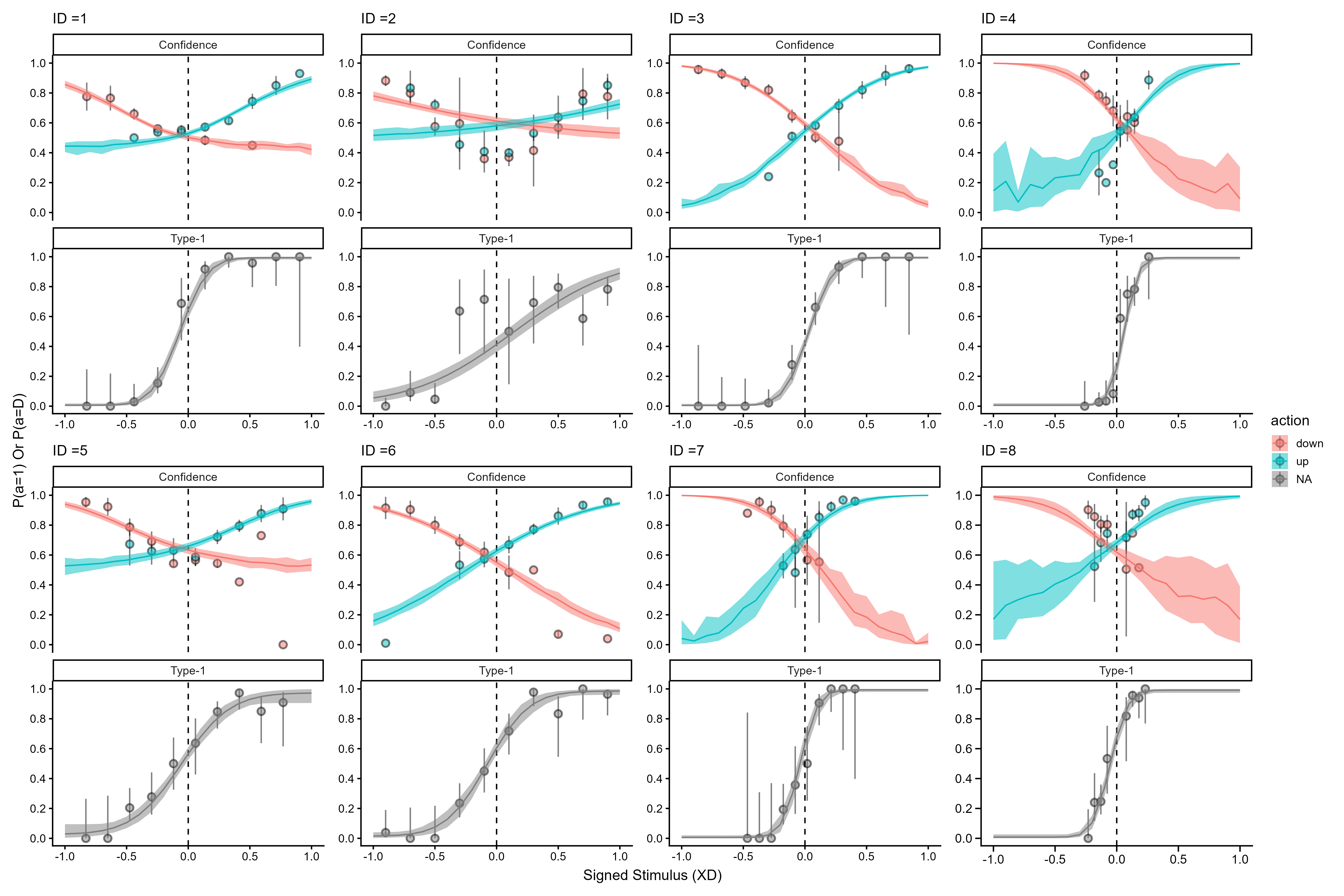
2.2.9 Posterior predictive checks
Next, we show posterior predictive checks of the hierarchical heuristic model for our pilot participants.
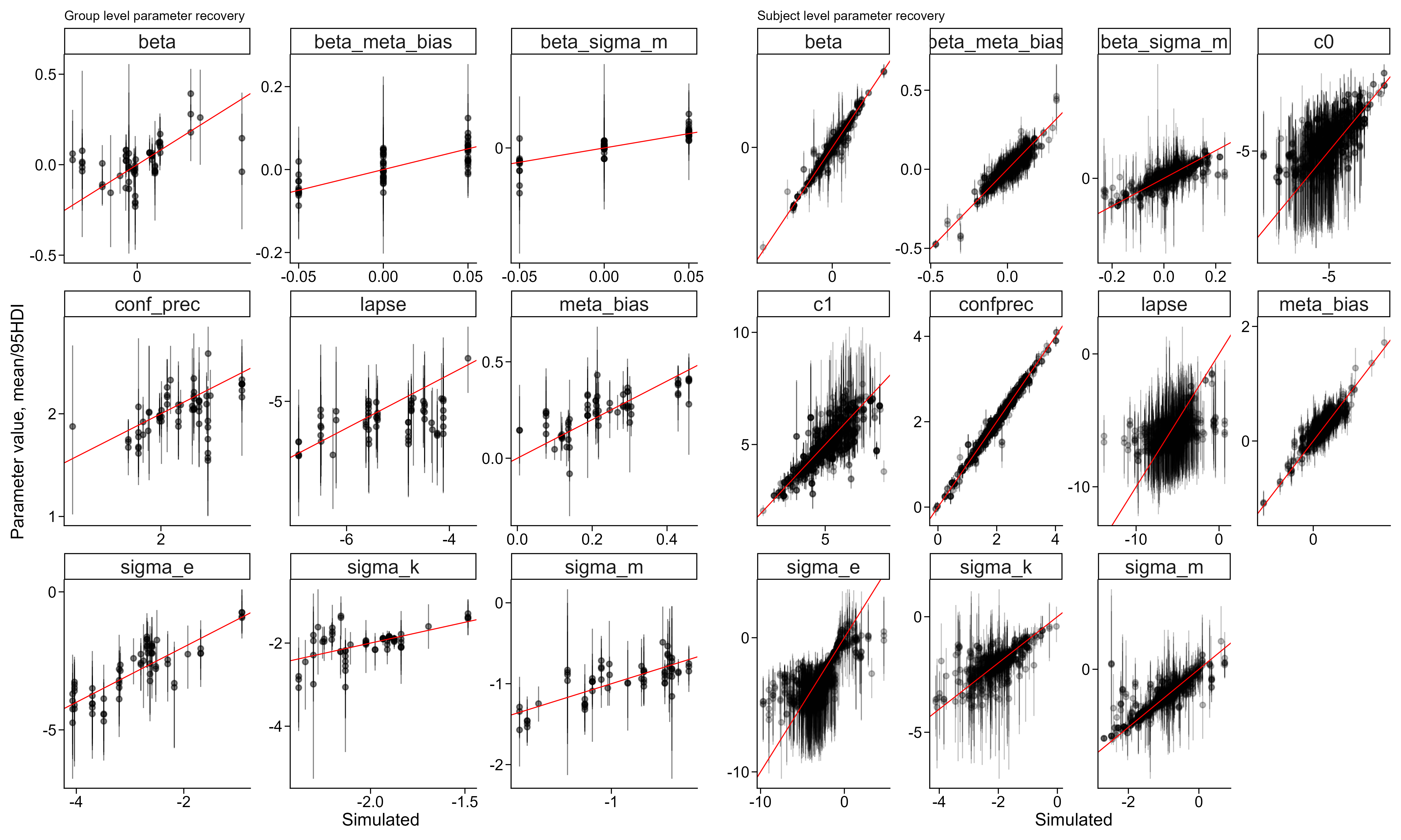
2.2.10 Hierarchical parameter recovery
To further assess the robustness of our model implementation and the planned sequential sampling procedure, we simulated new participants from the posterior distribution of the hierarchical model. We extracted a single posterior draw and simulated 25 participants from it, then fitted the model to increasing numbers of participants (5, 7, 9, 12, 15, 20, 25) to demonstrate that the sequential sampling approach is feasible. This also allowed us to perform parameter recovery on the hierarchical model without additional computational resources. Below, we show that the model adequately recovers its parameters at both the subject and group level for parameters of interest.
2.2.11 Sequential sampling
2.2.11.1 Priors
Because our sequential sampling approach uses Bayes factors for the termination of data collection, the prior distributions are highly influential. For transparency, we visualize the curves permitted by the prior below. Interested readers are also referred to the Sequential Sampling directory, which contains scripts for fitting, visualizing, and diagnosing our model.
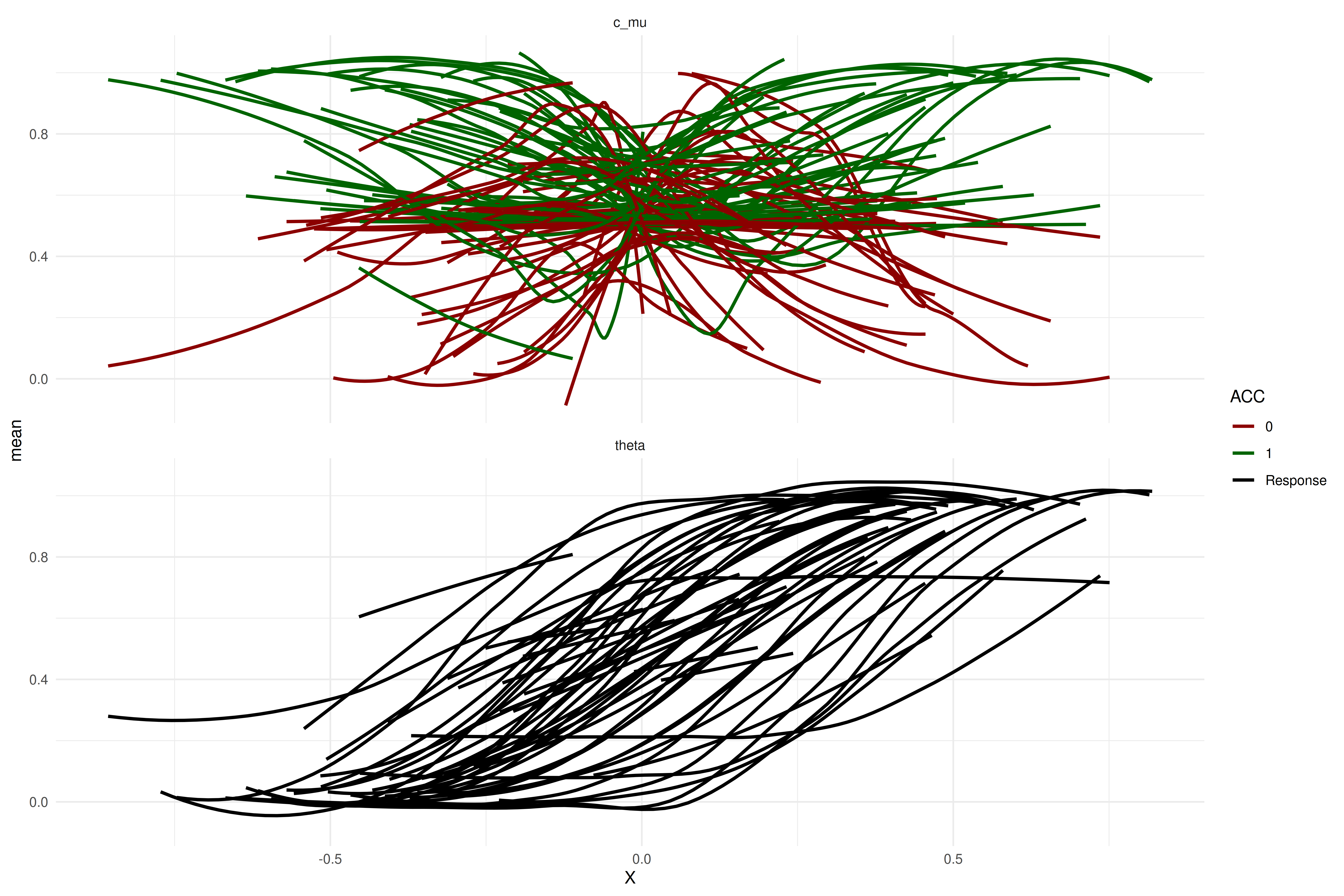
The plot above shows prior predictive checks of the group-level parameters (i.e., these curves represent group-level predictions). The curves span a wide range of possible patterns. To test whether our sequential sampling approach works, we simulate data from draws of the posterior distribution of our pilot data and examine how the Bayes factors for both hypotheses evolve as more participants are collected. Rather than using posterior draws of the parameters of interest (\(\mu_{\Delta{\sigma_{m_s}}}\) and \(\mu_{\Delta{\mu_{\beta_c}}}\)), we fixed these to \(-0.05\), \(0\), or \(0.05\) to test whether we can detect effects of this magnitude in both directions and also terminate sampling when the effect is zero. Below, we display the size of these effects (simulated from the mean of the group means).
As described above, we simulated participants from draws of the posterior informed by our pilot data. We then fitted the model to increasing numbers of participants (5, 7, 9, 12, 15, 20, 25) to demonstrate the feasibility of the sequential sampling approach. Below, we show five such trajectories of Bayes factors as a function of sample size, alongside a panel showing how the posterior distribution of the parameter of interest changes with increasing sample size.
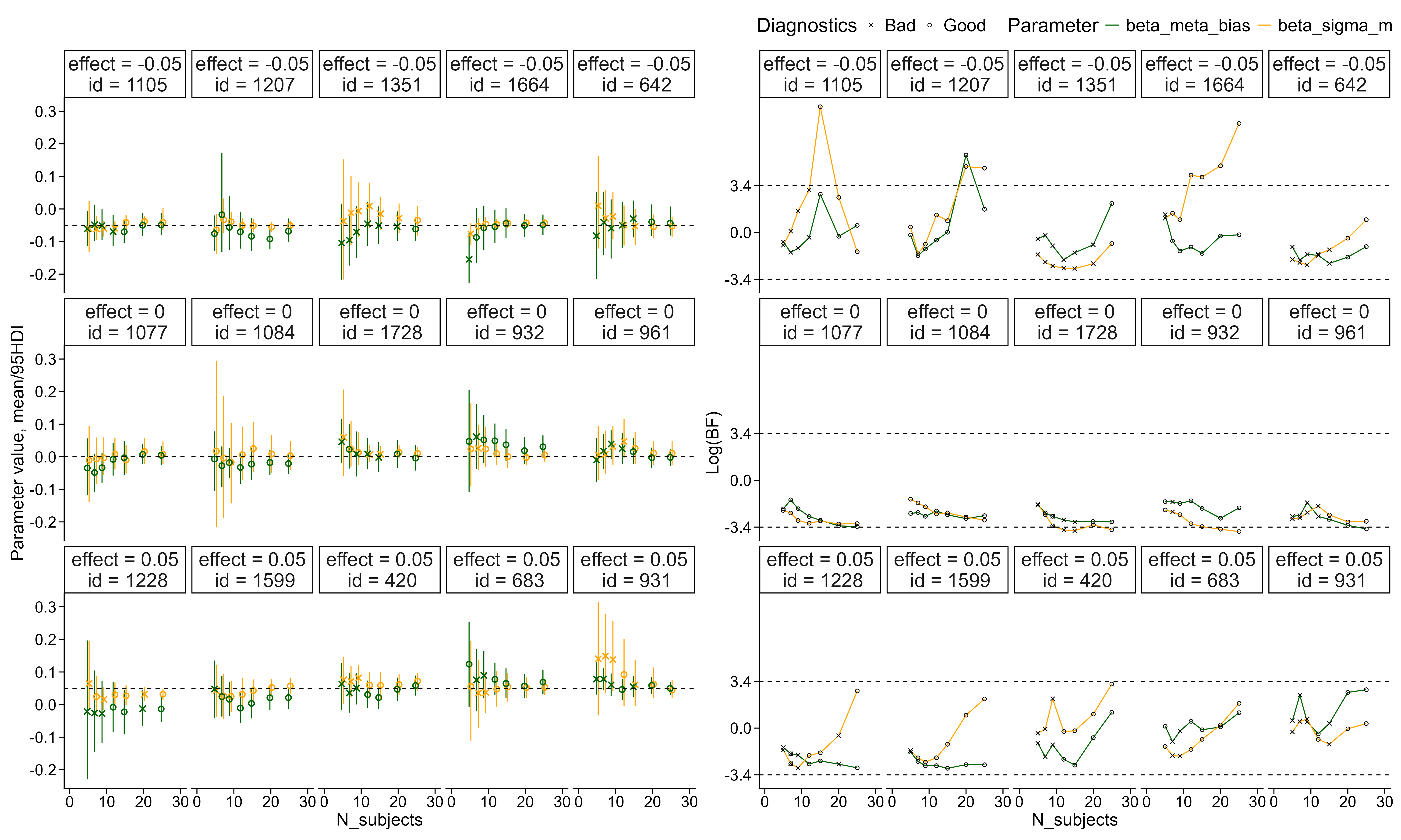
The above plot shows how the estimated effect of the interval between choice and confidence rating evolves for both metacognitive bias (green) and metacognitive noise (orange). Circles indicate fitted models without divergences, with effective sample sizes above 400 for both bulk and tails and \(\hat{R}\) values below 1.03. The left panel displays the posterior distribution of each parameter for increasing sample sizes. The right panel displays the corresponding Bayes factors for the same posterior draws fitted to our pilot data.
The above plot also shows that convergence issues may arise even with this model. Below, we describe our approach for identifying and handling convergence issues.
We will collect data from 15 participants before fitting the hierarchical model for the first time and testing the Bayes factor, because hierarchical models generally require a minimum amount of data to converge (see also the simulation above). After this initial fit, we will check the Bayes factor after each additional 5 participants, which coincides with the expected number of participants collected per day.